# USER HELP CENTER

This part will help you better understand Get3D's products and get started with them.

Our technology has been applied to many famous archaeological excavation sites, the digitization of World Heritage sites, the 3D Reconstruction of **Mega Cities**, **Large-scale Engineering Construction**, **Space Exploration**, and so on. In addition, we are integration 3D Reconstruction technology with AI to create innovative solutions. We continue to work on **Photogrammetry**, **SLAM**, and **AI-Related Technologies** to develop more convenient products for the Sensing, Measurement, and analysis of the Physical world, and to use technology to make life more convenient.


# Get3D Mapper

Scalable, rapid and highly accurate 3D modeling


# Basic Information

This section will introduce you to the Get3D Mapper software, and pre-use requirements.


# About Get3D Mapper

Scalable, rapid and highly accurate 3D modeling

*<mark style="color:yellow;">**Get3D Mapper**</mark>* is a **Large-scale** Photogrammetric 3D Cluster Modeling software for the professional mapping and general-mapping applications.

The software is a perfect combination of the latest research results in **Photogrammetry** and **Computer Vision**, and incorporates **Deep Learning** technology for intelligent processing, which can support 3D reconstruction from oblique photography. It is also compatible with large scale traditional aerial photography, close-range photography and laser point cloud processing. The software provides highly automated processing of Aerial Triangulation, 3D reconstruction and can generate highly accurate, high quality 2D Maps ( DSM / DOM) and 3D Products (standard 3D Model, point cloud products, etc.).


# Useful Concept

This section introduces you to some of the basic photogrammetric knowledge required to use Get3D Mapper, as well as the relevant terminology in the software.

<table data-view="cards"><thead><tr><th></th><th></th><th></th></tr></thead><tbody><tr><td><mark style="color:purple;background-color:purple;"><strong>Oblique Photogrammetry</strong></mark></td><td>Oblique photogrammetry is the simultaneous acquisition of surface images from multiple different viewpoints by flying a platform with a camera on board to obtain rich surface information for the production of mapping and geographic information products.</td><td></td></tr><tr><td><mark style="color:purple;background-color:purple;"><strong>Unmanned Aerial Vehicle (UAV)</strong></mark></td><td>It is an unmanned aircraft that can be equipped with different sensors and is operated by radio remote control equipment and its own program control device. The images captured by the UAV can be imported into the software for modeling.</td><td></td></tr><tr><td><mark style="color:purple;background-color:purple;"><strong>Close to Ground Photography</strong></mark></td><td>Obtain high-resolution lateral texture and structural details of features using mobile phones, digital cameras, handheld gimbals, vehicle-mounted mobile surveys, stationary laser scanning, or low-altitude ring photography.</td><td></td></tr><tr><td><mark style="color:purple;background-color:purple;"><strong>Pose File</strong></mark></td><td>A comprehensive representation of position (Position) and orientation (Orientation) in space, the Pose file is used to record information about the camera's position and pose when a photo is taken, recording the coordinates (x, y, z) of the position in three-dimensional space and the quaternion or rotation matrix of the camera's pose.</td><td></td></tr><tr><td><mark style="color:purple;background-color:purple;"><strong>Exif (Exchangeable Image File Format)</strong></mark></td><td>EXIF is a metadata standard embedded in image files and is primarily used to store information about the image taken. This information includes shooting time, exposure settings, white balance, camera model, focal length, geographic coordinates, and so on.</td><td></td></tr><tr><td><mark style="color:purple;background-color:purple;"><strong>Image</strong></mark> <mark style="color:purple;background-color:purple;"><strong>Control Point</strong></mark></td><td>Image Control Points are control points measured in the field for the densification of photogrammetric and mapping control. They include plane control points (with plane coordinates only), elevation control points (with elevation only), and combined control points (with both plane coordinates and elevation).</td><td></td></tr><tr><td><mark style="color:purple;background-color:purple;"><strong>Ground Sampling Distance(GSD)</strong></mark></td><td>Ground resolution, which represents the actual size of the ground (usually measured in metres) represented by one pixel (Pixel), and is related to the pixel size of the image and the height of the camera at the time of imaging, etc. GSD = (P×H)/F P represents the pixel size (in metres per pixel), H represents the camera height (in metres), and F represents the focal length of the camera (in millimetres).</td><td></td></tr><tr><td><mark style="color:purple;background-color:purple;"><strong>Tile</strong></mark></td><td>3D model results are generally stored in a certain grid size, with individual grids called tiles. When large-scale 3D scene, processing the whole scene or terrain as a whole may lead to the problem of large amount of individual model data and low processing efficiency. Each tile represents a localised area that can be independently reconstructed in 3D. This chunking approach can significantly reduce the amount of data for a single processing task and can support distributed computing of tasks to improve processing speed. Tile technology also makes data transmission, storage and display more efficient.</td><td></td></tr><tr><td><mark style="color:purple;background-color:purple;"><strong>Relative Orientation</strong></mark></td><td>Relative orientation refers to the work of restoring or determining the relative relationship between pairs of images at the time of photography, i.e., the work of solving the relative orientation elements of stereoscopic pairs. It is to determine the internal and external parameters of the camera by observing the positional relationship of the objects in the image in different viewpoints. The relative orientation of stereo image pairs is to restore the interrelationship of the two neighbouring image beams at the time of photography, so as to make the pairs of light rays of the same name intersect each other.</td><td></td></tr><tr><td><mark style="color:purple;background-color:purple;"><strong>Absolute Orientation</strong></mark></td><td>Absolute orientation is the linking of an image to a ground coordinate system through measurements with ground control points. With the help of known ground control points, it translates, rotates, and scales the three-dimensional geometrical model, which has been relatively orientated, to incorporate it into the ground photogrammetric coordinate system. In this way, we can obtain the true position of objects on the ground.</td><td></td></tr><tr><td><mark style="color:purple;background-color:purple;"><strong>Camera Internal Orientation</strong></mark></td><td>The internal orientation (or internal parameters) of a camera refers to a number of internal properties of the camera: the sensor size of the camera, the focal length of the lens, the position of the principal points in the image plane, and the lens distortion. We call a group of images a set of images with identical internal orientations. For a physical camera with all settings fixed, the internal orientation is unique. Even for two cameras of the same model with the same settings, their respective images do not constitute a single image group.</td><td></td></tr><tr><td><mark style="color:purple;background-color:purple;"><strong>Tie Point</strong></mark></td><td>Tie Points are used for neighbouring models to connect image points with the same name.</td><td></td></tr></tbody></table>


# System Requirements

Computer requirements and recommended configuration for using Get3D Mapper.

## Operating System Requirements

<table><thead><tr><th>Supported Windows Operating Systems for Get3D Mapper</th><th data-hidden></th><th data-hidden></th></tr></thead><tbody><tr><td>Windows Server 2012 (x64)</td><td></td><td></td></tr><tr><td>Windows 10 (x64)</td><td></td><td></td></tr><tr><td>Windows 11 (X64)</td><td></td><td></td></tr><tr><td>Windows Server 2016</td><td></td><td></td></tr><tr><td>Windows Server 2019</td><td></td><td></td></tr></tbody></table>

## Graphics Card Requirements

Supports NVIDIA series discrete graphics cards with at least 4GB of GPU memory, CUDA version 12.5 or newer. And NVIDIA GPU is necessary for Get3D Mapper.

<mark style="color:purple;background-color:purple;">**The software CANNOT support AMD GPU for 3D modeling.**</mark>

How to check NVIDIA graphics card driver version and CUDA version:

<figure><img src="/files/Dox4YnQq8vKhk94umKlK" alt=""><figcaption><p>NVIDIA System Information</p></figcaption></figure>

## Hardware Recommendation

* Operating System: Windows 10/11 (64 bit)&#x20;
* RAM: 64GB
* GPU: NVIDIA GeForce RTX 30 series or Higher
* VRAM: 8GB
* CPU Intel K-series CPU or AMD CPU with high base frequency


# Data Formats

This chapter introduces you to the input data formats and output result formats supported by Get3D mapper.

## Data Input

**Image Formats:** TIFF, JPEG,JPG

**Video Formats:** MP4, WMV, AVI, MOV

**Point Cloud File Formats:** LAS, PTX, PTS, E57

**Pose File Formats:** TXT, CSV

**Boundary File Format:** KML

**Block File Formats:** XML, XBIN

## Data Output

### 3D Model

The data formats supported by Get3D Mapper for creating 3D models include OBJ format and OSGB format. Both of the following data formats are supported to be opened in Get3D Viewer software.

**①　OBJ (Wavefront OBJect):**&#x20;

OBJ format is a file format for representing 3D geometric objects. It contains information that describes the geometry of a 3D object, and its file consists of polygonal faces that are further defined by elements such as vertices, normals, curves, texture maps, and surfaces etc. An OBJ file is a vector file that is scalable and has no maximum file size limit. Due to its simplicity and readability, it has become a widely used format for exchanging 3D models.

**②　OSGB (Open Scene Graph Binary):**&#x20;

The OSGB format is a binary file format in the framework of OpenSceneGraph (OSG), an open source, cross-platform, high-performance 3D graphics toolkit, and OSGB is the file format it uses to store and load 3D models and associated material, texture, and geometry data. The OSGB format uses a binary format and uses compression algorithms and data structure optimization to reduce file size and improve loading performance. This makes OSGB format perform well when dealing with large 3D models and complex scenes, making it an ideal choice for storing and representing 3D scene graphics data.

Overall, OBJ format is mainly used to represent the geometry and texture information of 3D models, while OSGB format focuses on the efficient storage and loading of 3D models, which is especially advantageous when dealing with large and complex scenes. When loading 3D models with Get3D Viewer, it is recommended to use OSGB format to preview the model faster.

### Point Cloud

Get3D Mapper supports the generation of 3D point cloud data converted from 3D models or dense matches in \*.las, \*.txt, \*.asc, and \*.e57 formats.

**①　.las format (Lidar Aerial Survey) ：**

The .las format is a commonly used point cloud data format developed by the U.S. Geographic Survey (USGS) and U.S. partners. It is primarily used to store point cloud data acquired by LiDAR scanners, including geometric information (e.g., coordinates, intensities, etc.) as well as other metadata (e.g., scanning parameters, classifications, etc.) for the point cloud.The LAS file is saved in a binary format consisting of a file header that contains the metadata, and a series of point records that contain information specific to each point.

**②　 .txt Format (Text File)：**

&#x20;The .txt format is a simple representation of point cloud data, which saves the point cloud data as a plain text file. In this format, each line usually represents the location and color information of a point, making the data easy to read and process, but may not be suitable for storing large or complex point cloud data.

**③　 .asc format (ASCII) .asc format, or ASCII format：**

&#x20;is a text file format. In this format, point cloud data is stored as visual text.The ASC model format was developed by Autodesk to make it easier to exchange 3D data between various 3D modeling software. It makes it simple to transfer and share data between different software platforms.

**④　.e57 Format:**&#x20;

The E57 format is an open-source, compact and vendor-neutral format developed by ASTM International's 3D Imaging Data Committee. It uses a combination of binary and XML formats to store data such as that acquired by laser scanners, radar (LADAR), and optical rangefinder cameras (Flash LADAR) and LIDAR images.The content of E57 files is encoded in a hierarchical tree structure using an optimized subset of XML, which allows for the efficient storage of large amounts of binary data, making it ideally suited for the exchange of 3D imaging data. .

Each of these formats has its own features and advantages in point cloud data processing, storage and exchange, and users can choose the appropriate format for their specific needs.

### 2D Data

Mapper supports the generation of planar 2D topographic maps including DOM and DSM.

**①　DOM (Digital Orthophoto Map):**&#x20;

It is the image data generated by using the digital elevation model on the scanned and processed digitized aerial film/remote sensing image (monochrome/color), correcting the projection difference pixel by pixel, and then cropping the image data according to the image mosaic according to the range of the image format.The principle of DOM production is to apply the professional geographic information remote sensing software to the original remote image after radiometric correction and geometric correction according to its characteristics. The principle of DOM production is to apply professional geographic information remote sensing software to the original remote sensing image after radiometric correction and geometric correction to eliminate all kinds of aberrations and displacement errors, and finally get the satellite remote sensing digital orthophoto maps that contain geographic information and various topics.DOM has the image with a certain geometric accuracy. DOM has a certain geometric accuracy, complete and full vegetation information, clear and uniform overall color tone, and moderate contrast.

**②　DSM (Digital Surface Model)：**&#x20;

DSM is a digital model that represents the elevation information of the ground surface and the objects above it (e.g. buildings, trees, utility poles, etc.). It includes the elevation data of the ground surface and these obstacles, so it can more realistically reflect the shape of the ground surface.DSM can be used to produce 3D models, remote sensing analysis and many other applications.


# Getting Started

This section will guide you on how to use Get3D Mapper.


# Newbie Guide

Here we take a piece of data as an example to show you the whole process from images to model.

## 1 Download & Installation

Login to the official website [www.get3d.ai](https://www.get3d.ai/), go to the download page to download the software executable program Get3D Mapper.exe, as well as the demo data. Under Windows operating system, double-click the program to load it and install it automatically. After the installation is completed, a shortcut with the software icon will be displayed on the Windows desktop, and you can open the software by double-clicking it.

<figure><img src="/files/qvUKoBWl7bddP87Q3NTE" alt=""><figcaption><p>Download</p></figcaption></figure>

## 2 License Acquisition

After entering the Get3D Mapper software interface for the first time, you need to obtain a license to use the software for modeling.

There are two types of licenses: trial and official.&#x20;

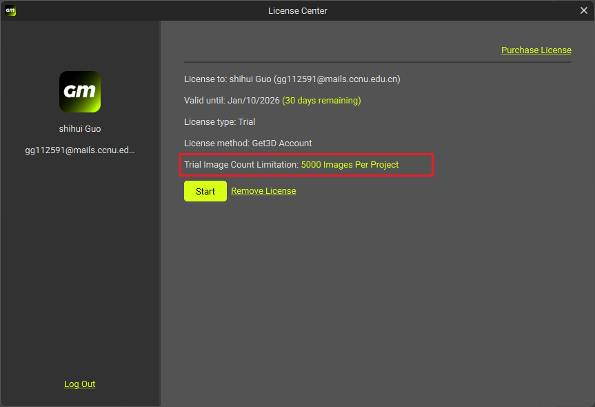
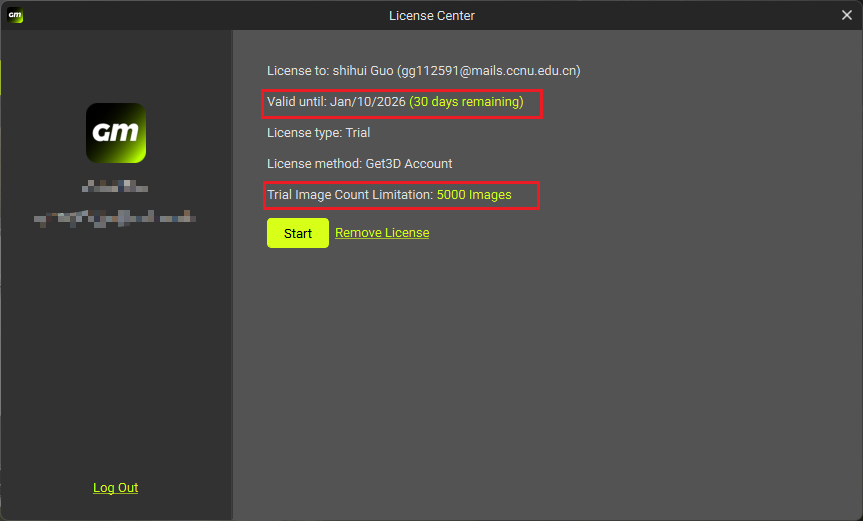
* Trial license: After registering an account, you will automatically get a trial license, which can be activated online or offline and is valid for one month from the activation date.  Trial license supports unlimited project creation within 30 days, and a single project can import 5,000 images.

{% hint style="warning" %}
After version 7.0.9, both trial and official licenses are activated online or offline, and there is no separate activation interface for trial license.
{% endhint %}

<figure><img src="/files/bsIEXSjuufVNS8bHG2Uk" alt=""><figcaption><p>Trial License</p></figcaption></figure>

* Official license: An official license is obtained through purchase and can be subscribed monthly or annually. Select the available license to activate, the activated license will show the expiry time, all the functions can be used during the period, and there's no limit for image count.

<figure><img src="/files/HpDwbfK3JmHTvkK3R7iJ" alt=""><figcaption><p>Official License</p></figcaption></figure>

Both trial and official licenses can be activated online or offline.

### 2.1 Online Activation

#### Get3D Account

Login Get3D account, you can get all the historical license information about Get3D Mapper software under that account. The available license information includes the license ID, the activation status of the ID, the valid of the license period, and the expiration date. Select available license to activate.

1. Log in Get3D account.

<figure><img src="/files/ceAVuJqxTAX3U83phrS9" alt=""><figcaption><p>Get3D Account Mode</p></figcaption></figure>

<figure><img src="/files/GBmDZuD4bvZNV8xMGhMj" alt=""><figcaption><p>Login</p></figcaption></figure>

2. Refresh license list.&#x20;
3. Select one license to be activated.&#x20;
4. click **Activate** button to activate it.

<figure><img src="/files/UzPOr8YvDewkxtPdNBMe" alt=""><figcaption><p>Activate License</p></figcaption></figure>

### 2.2 Offline Activation

#### License Document Mode

The other way to activate the official license applies when the PC is offline.

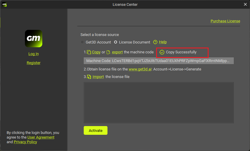
Firstly, **export** the machine code, and then in the personal account center on the web side, input the machine code to get the license file. Import the **license file** to the software and click **Activate** to complete the binding of machine code and license.

1. **Copy** or **Export** machine code.

<figure><img src="/files/3tfJHhiCzdygbJSNZTnK" alt=""><figcaption><p>Copy Machine Code</p></figcaption></figure>

<figure><img src="/files/CrfJPdvhMs6sWy3CKvIp" alt=""><figcaption><p>Export Machine Code</p></figcaption></figure>

2. Open the website [license center](https://www.get3d.ai/personal-center/license).

<figure><img src="/files/amtpKTDoOS1O1ItY13pR" alt=""><figcaption><p>Get3D Website</p></figcaption></figure>

3. Select one license and click **Generate.**

<figure><img src="/files/7REpDr3CSS03dM6LZTZA" alt=""><figcaption><p>Personal Center</p></figcaption></figure>

4. **Upload** machine code and **download** license file.

<figure><img src="/files/vKukzWywAqsO3l3lyBxC" alt=""><figcaption><p>Obtain License</p></figcaption></figure>

5. Import license file and click **Activate** button.

<figure><img src="/files/iQSsHtggt5mDQjoeVjLe" alt=""><figcaption><p>Import and Activate License</p></figcaption></figure>

Activated license information can be viewed in License Center.

<figure><img src="/files/9AWUysMIdzSSs70sh5Fy" alt=""><figcaption></figcaption></figure>

### 2.3 License Information Management

For users who have already purchased the official version of the license, you can go to the official website personal center to view the complete license information and purchase history orders.

<mark style="color:purple;background-color:purple;">**Note: Once the license activated, it can't be transferred to other computer. The license is bound to machine.**</mark>

## 3 Create Project & Open Project

When use the software for the first time, click **New Project** to generate a project folder containing .m3d project files. When you open the project later, you can double click the .m3d file directly.

<figure><img src="/files/R7H1lTp4Qjdt9xzaGS2g" alt=""><figcaption><p>Create a New Project</p></figcaption></figure>

<figure><img src="/files/TffBxhNncvBZcUt85Sew" alt=""><figcaption><p>Open Project</p></figcaption></figure>

## 4 Import Image

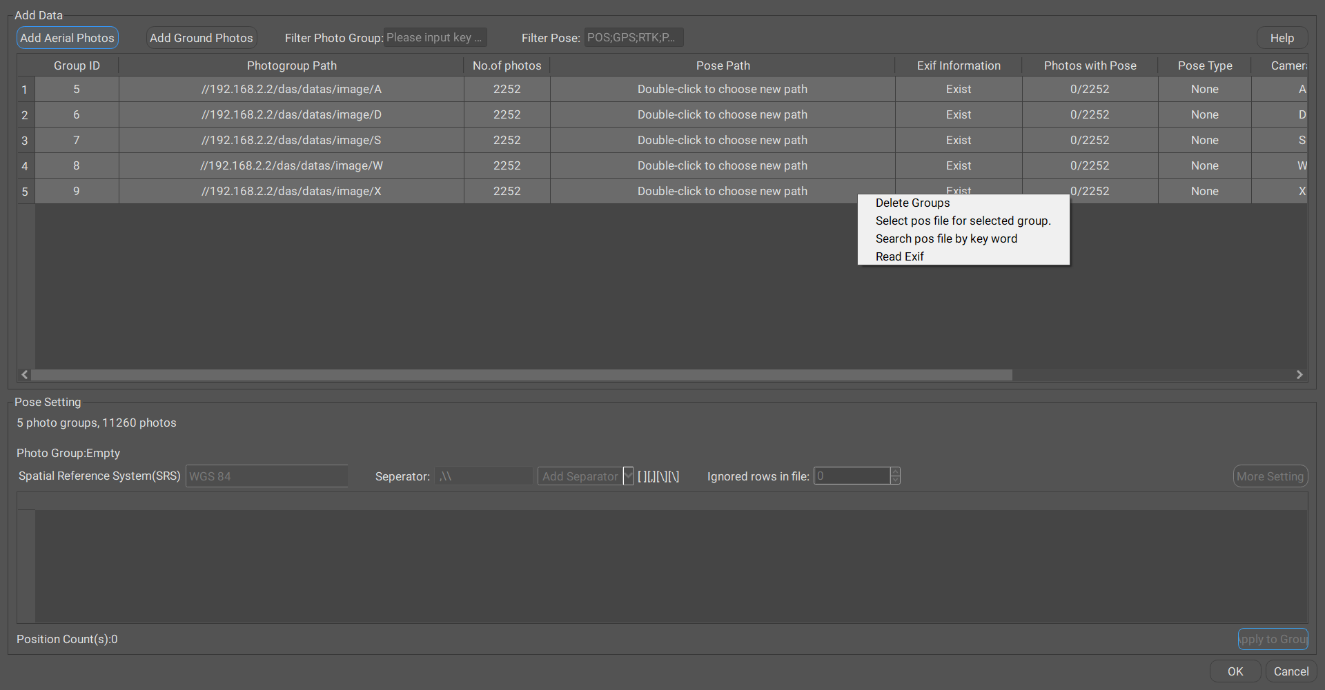
In the **Data Prepare** page where you can import data, click **Add Photos** to open the **Import Photo Pose Setting** window.

<figure><img src="/files/tb4qVFOJPz9VQ8wVEsdm" alt=""><figcaption></figcaption></figure>

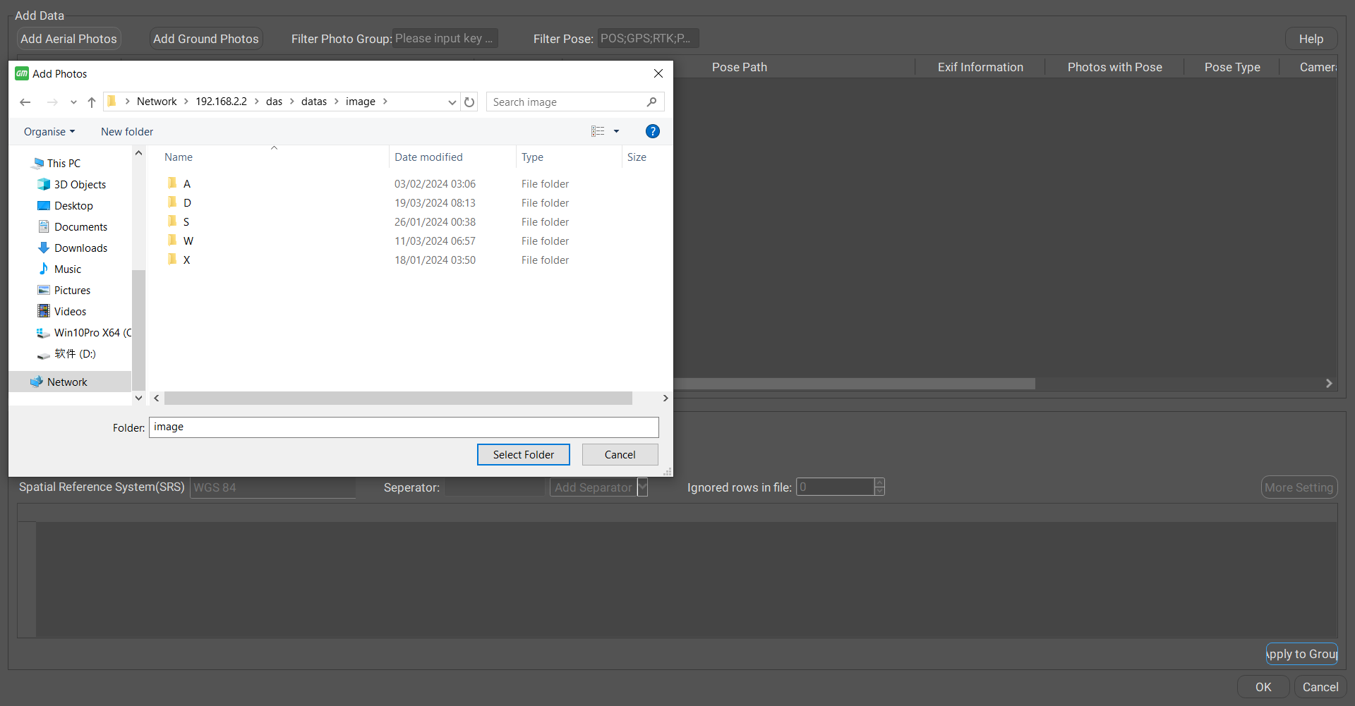
&#x20;Click **Add Aerial Photos** to import the data folder into the software.

<figure><img src="/files/fF5RKlxE6RzbdhjoWMci" alt=""><figcaption><p>Select Folder</p></figcaption></figure>

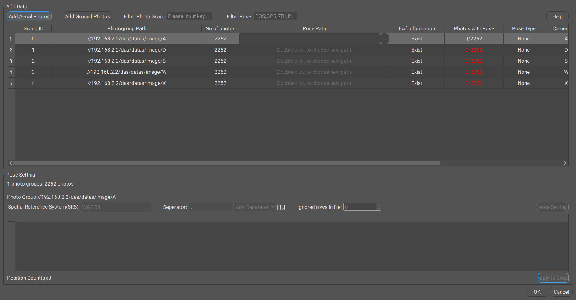
After importing, the interface before positioning is as follows:

<figure><img src="/files/zCMPIftcXOEcd1NCbSAS" alt=""><figcaption></figcaption></figure>

## 5 Photo Positioning

There are two ways to position imported images.

### 5.1 Pose File Positioning

The first way of positioning is based on the pose file. Select the photo group, right click and choose pose file positioning, import pose file.

<figure><img src="/files/gubTCHmgImvmExwzbBym" alt=""><figcaption><p>Select Pose File</p></figcaption></figure>

For the photos after importing the pose file, select any group and the pose setting screen will appear below.

Select the correct Spatial Reference System to correspond each column of data to its coordinate system units.

Then click **Apply to Photo Group**.

<figure><img src="/files/LnD6N7XjGGktRKTwtXze" alt=""><figcaption><p>Set Parameters</p></figcaption></figure>

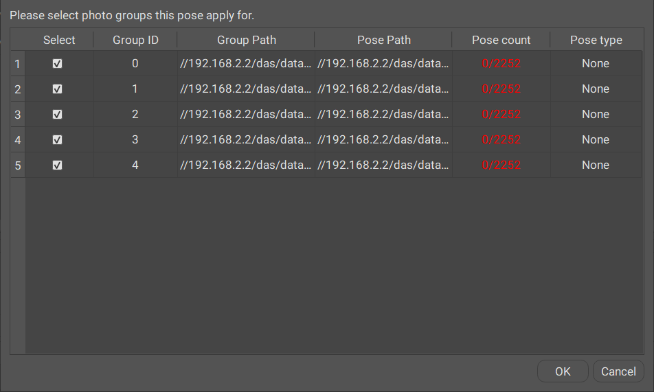
Select the group to correspond to and click **OK**.

<figure><img src="/files/RwceAZZYd8C4kYHFsNkL" alt=""><figcaption><p>Correspond to Photo Group</p></figcaption></figure>

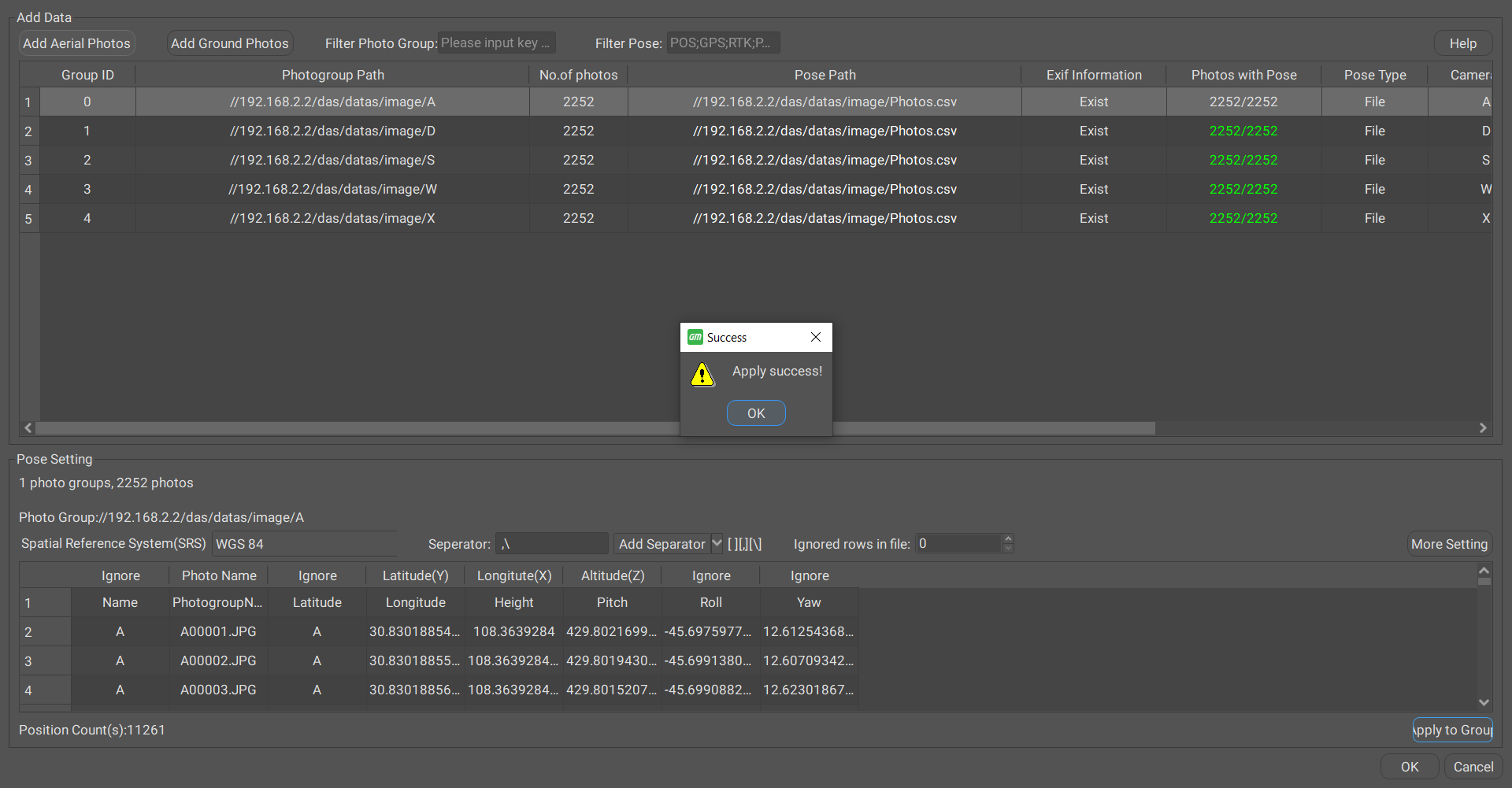
If successful, the following window appears.

<figure><img src="/files/yZHoSHkgMuuyfJO4pnDP" alt=""><figcaption><p>Apply Successfully</p></figcaption></figure>

Click **OK** to complete the photo import and positioning.

<figure><img src="/files/SMHUg5tdY2JsywgvcXLV" alt=""><figcaption><p>After Positioning</p></figcaption></figure>

Tutorial video: <https://youtu.be/1oA6RwfNr54?si=kHVPP4TisYzzvJZ6>

### 5.2 EXIF positioning

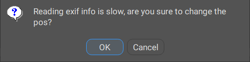
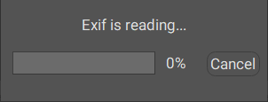
Select the photo group that **Exif Information** exist, right-click and select **Read Exif** to give photos position.

<figure><img src="/files/o9ygbvq0yqKcUa54C7af" alt=""><figcaption><p>Read EXIF</p></figcaption></figure>

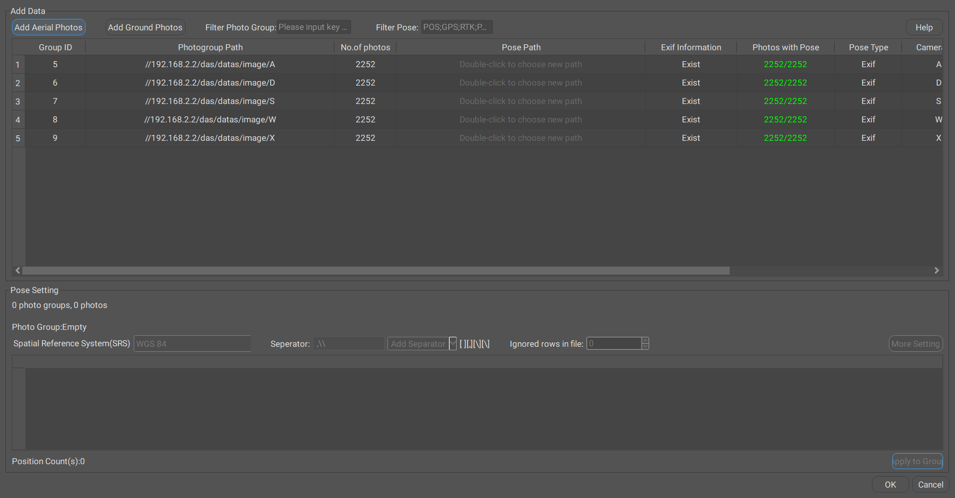
If successful, Photos with Pose value will change to green. The interface after successful positioning is as follows:

<figure><img src="/files/bx1EJoUmc2waZ4hh4FcQ" alt=""><figcaption><p>Positioning Successfully</p></figcaption></figure>

Click "OK" finish importing and positioning photos.

<figure><img src="/files/IcluoFlLoo09A93X2Ucr" alt=""><figcaption><p>After Positioning</p></figcaption></figure>

## 6 Job Queue & Engine Setting

When the photo positioning is finished, click Apply in the bottom right corner to save the block.

<figure><img src="/files/hGH2s3UKQauSFJPWj1VH" alt=""><figcaption><p>Data Prepare Interface</p></figcaption></figure>

Click **Setting** on the top menu bar to open the Job and Engine Setting window.

<figure><img src="/files/nc2Tmqve3eRkRDRsSIgY" alt=""><figcaption><p>Setting</p></figcaption></figure>

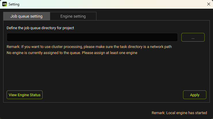
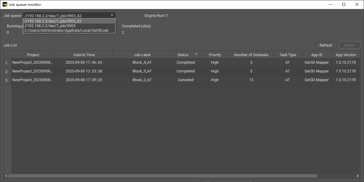
Set the **job queue directory** for project and click **Apply**.

<figure><img src="/files/rrTOvzp9gH7cgsXvbUsj" alt=""><figcaption><p>Job Queue Setting</p></figcaption></figure>

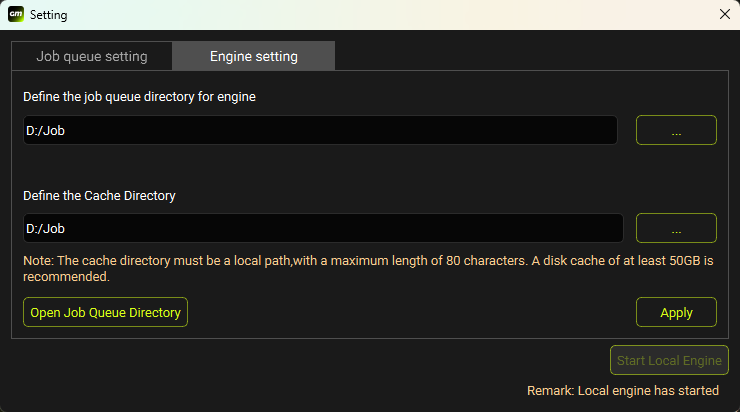
Set the **job queue directory** for engine and set **cache directory**, click **Apply**.

<figure><img src="/files/D6yrnvuhP9jsXkl7irpi" alt=""><figcaption><p>Engine Setting</p></figcaption></figure>

&#x20;After applying the paths, click **Start Local Engine** to open the Engine screen.

<figure><img src="/files/cUrbhQSwbTAyNcME2V6e" alt=""><figcaption><p>Start Local Engine</p></figcaption></figure>

{% hint style="info" %}
Job queue directory setup is optional. For first time users, you can directly **Start Local Engine**.
{% endhint %}

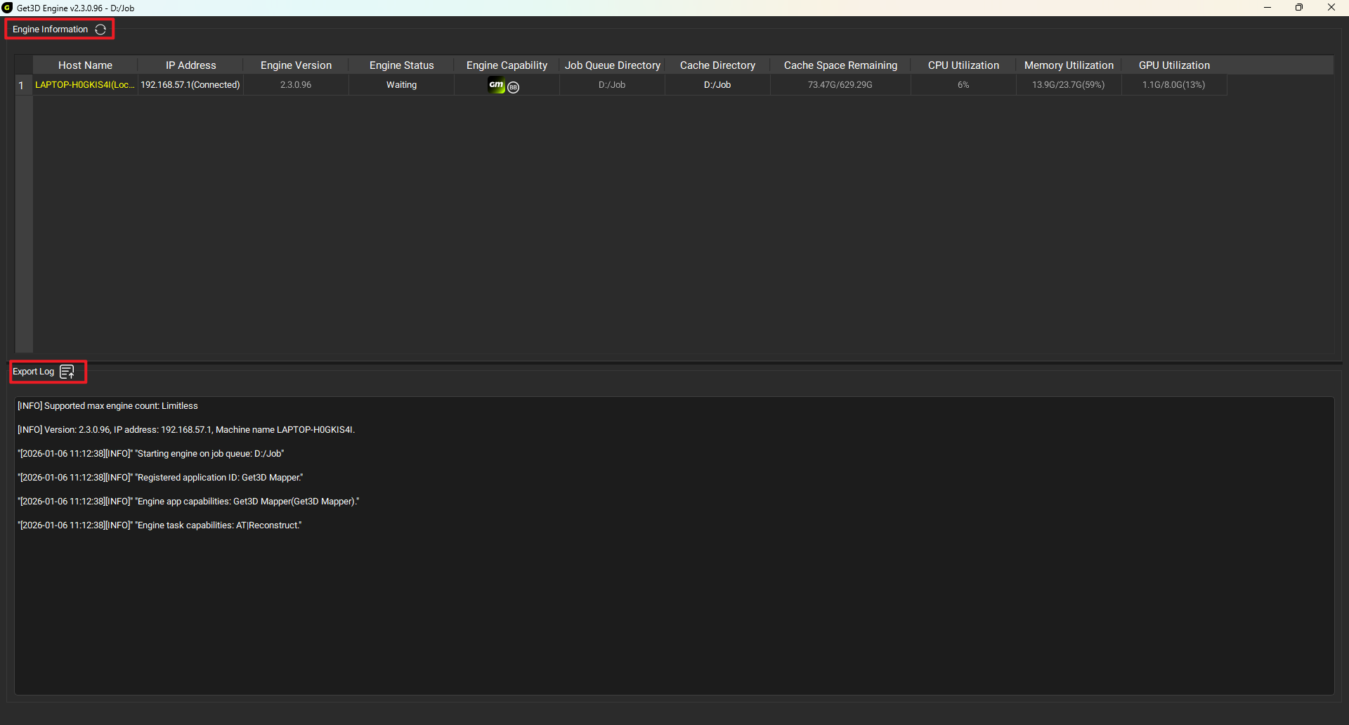
The engine status is **Waiting** when no jobs have been submitted. Engine specific information can be viewed in the Engine window.

<figure><img src="/files/AJPfXVI4URUQaC0f8f1X" alt=""><figcaption><p>Engine Interface</p></figcaption></figure>

## 7 Aerial Triangulation

Once the Engine Setting is complete, you can click **Submit AT**. If you do not fill in the sensor parameters and focal length information, a prompt box will pop up, select Fill to fill in the camera information.

<figure><img src="/files/ic8V2ugpTanPL1SaW8RO" alt=""><figcaption><p>Submit AT</p></figcaption></figure>

Fill in the correct sensor parameters and focal length information according to the camera model.

Note there is a difference between the focal length of the lower view lens and the focal length of the side view lens, please fill in correctly.

<figure><img src="/files/SyaLZDb9PQR2Qymt0nkh" alt=""><figcaption><p>Set Camera Parameters</p></figcaption></figure>

Once the camera information is filled in, continue back to the **General** view and click **Submit AT** to open the AT Settings window, click **Submit**.

<figure><img src="/files/UrtaqIMuac8ivmdXgRxT" alt=""><figcaption><p>Submit</p></figcaption></figure>

Aerial Triangulation is submitted, calculations pending...

<figure><img src="/files/yvrVRSRD6SeDJEoyvjRQ" alt=""><figcaption><p>AT Running</p></figcaption></figure>

At the end of Aerial Triangulation, the generated point cloud model can be viewed in the 3D view

<figure><img src="/files/YjoAXlmCVGt9luMX6kxX" alt=""><figcaption><p>Block 3D View</p></figcaption></figure>

Tutorial video: <https://youtu.be/dEJZR1Qh178?si=mFj2IvCOIZVV6ved>

## 8 Reconstruction

### 8.1 3DGS Reconstruction &#x20;

For blocks that have completed Aerial Triangulation calculations, right-click block and select **New 3DGS Reconstruction** or click the **New 3DGS Reconstruction** in the right bottom side to enter the Reconstruction screen.

<figure><img src="/files/QtRX3gOXqbXWFhb6GqJQ" alt=""><figcaption><p>Create New 3DGS Reconstruction</p></figcaption></figure>

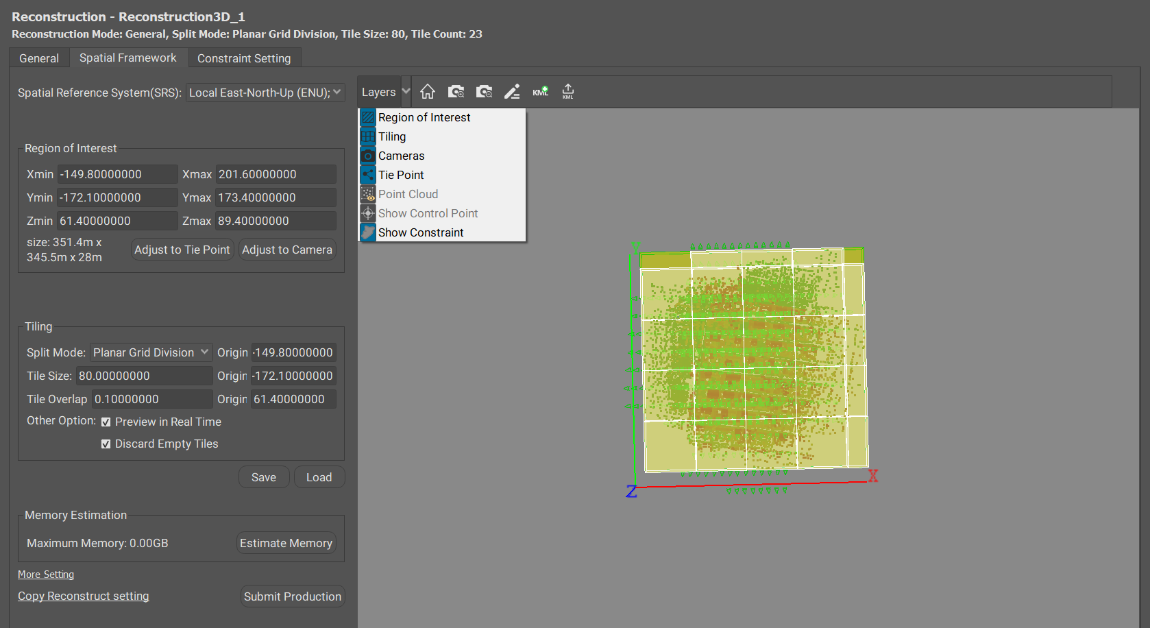
In the Reconstruction Settings screen, you can perform operations such as selecting Coordinate System and setting the width of each modeling’s tile.

<figure><img src="/files/ijsOI8vLrX3tsTwqDUjm" alt=""><figcaption><p>Set Reconstruction Parameters</p></figcaption></figure>

By clicking **Submit Production**, you can select the type of production you want to output. Get3D Mapper supports many types of production output.

<figure><img src="/files/QXdSe9mTAamnt3cILyvv" alt=""><figcaption><p>Select Product Type</p></figcaption></figure>

Click on **Select Tiles** to selectively model parts of the entire interior of the area.

<figure><img src="/files/jypZI0bDUgF6iBURumRs" alt=""><figcaption><p>Select Tiles</p></figcaption></figure>

After all the settings are done, you can click **OK** to submit the production and enter the reconstruction calculation.

<figure><img src="/files/Zfum9LEWiFX47nOANgtw" alt=""><figcaption><p>Production Running</p></figcaption></figure>

You can view the product and open it in **Get3D Viewer** with one click after merging the root node.

<figure><img src="/files/D7shRfi5AW8ZfHw7vxdi" alt=""><figcaption><p>Link Get3D Viewer</p></figcaption></figure>

Tutorial video: <https://www.youtube.com/watch?v=sWmk4LgOShQ>

### 8.2 3D Reconstruction &#x20;

For blocks that have completed Aerial Triangulation calculations, right-click block and select **New 3D Reconstruction** or click the **New 3D Reconstruction** in the right bottom side to enter the Reconstruction screen.

<figure><img src="/files/0hdFzq60lcoxbDsCGdVQ" alt=""><figcaption><p>Create New 3D Reconstruction</p></figcaption></figure>

In the Reconstruction Settings screen, you can perform operations such as selecting Coordinate System and setting the width of each modeling’s tile.

<figure><img src="/files/ijsOI8vLrX3tsTwqDUjm" alt=""><figcaption><p>Set Reconstruction Parameters</p></figcaption></figure>

By clicking **Submit Production**, you can select the type of production you want to output. Get3D Mapper supports many types of production output.

<figure><img src="/files/3IGkxWzNWoKUf0bfmBZW" alt=""><figcaption><p>Select Product Type</p></figcaption></figure>

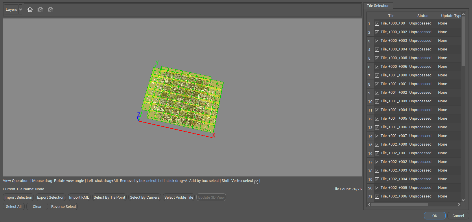
Click on **Select Tiles** to selectively model parts of the entire interior of the area.

<figure><img src="/files/1JfDxmi86S1NWBtjA3LZ" alt=""><figcaption><p>Select Tiles</p></figcaption></figure>

After all the settings are done, you can click **OK** to submit the production and enter the reconstruction calculation.

<figure><img src="/files/CgpzxOZM1MFLtGT3t9eM" alt=""><figcaption><p>Production Running</p></figcaption></figure>

After modeling, you can click **3D View** to view the modeling effect within the Mapper software interface.

<figure><img src="/files/YNmodCOqYAvZ36Vp3aPW" alt=""><figcaption><p>Model 3D VIew</p></figcaption></figure>

You can also choose to view the product and link **Get3D Viewer** software with one click to view the model.

<figure><img src="/files/D7shRfi5AW8ZfHw7vxdi" alt=""><figcaption><p>Link Get3D Viewer</p></figcaption></figure>

Tutorial video: <https://youtu.be/-Sgab5bIqT4?si=XXdSR_1r_X54wXcK>

### 8.3 2D Reconstruction

Right-click block and select **New 2D Reconstruction** or click the **New 2D Reconstruction** in the right bottom side to enter the Reconstruction screen.

<figure><img src="/files/kS2wHodTNN3kwwn54aPA" alt=""><figcaption><p>Create New 2D Reconstruction</p></figcaption></figure>

In the Reconstruction Settings screen, you can perform operations such as selecting Coordinate System and setting the width of each modeling’s tile.

<figure><img src="/files/BVbhyKC25sIWoD3J7yAl" alt=""><figcaption><p>Set Reconstruction Parameters</p></figcaption></figure>

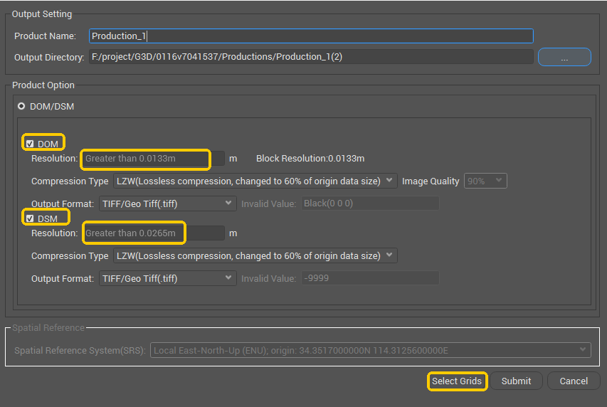
By clicking **Submit Production**, you can select the type of 2D production you want to output. DOM and DSM product are supported in 2D reconstruction. Set the resolution for DOM/DSM.

<figure><img src="/files/xF61qJVxjd73fhkkSbzD" alt=""><figcaption><p>Select Product Type</p></figcaption></figure>

If the Merge DOM and Merge DSM options are selected, an additional "MergeDomDsm" folder will be generated in the output, containing the merged DOM and DSM results.

<figure><img src="/files/XZnhtD6UIKTxiQNicRkc" alt=""><figcaption><p>Merge DOM/DSM </p></figcaption></figure>

<figure><img src="/files/nsOySuZa2QIMNKwwciz0" alt=""><figcaption><p>MergeDomDsm</p></figcaption></figure>

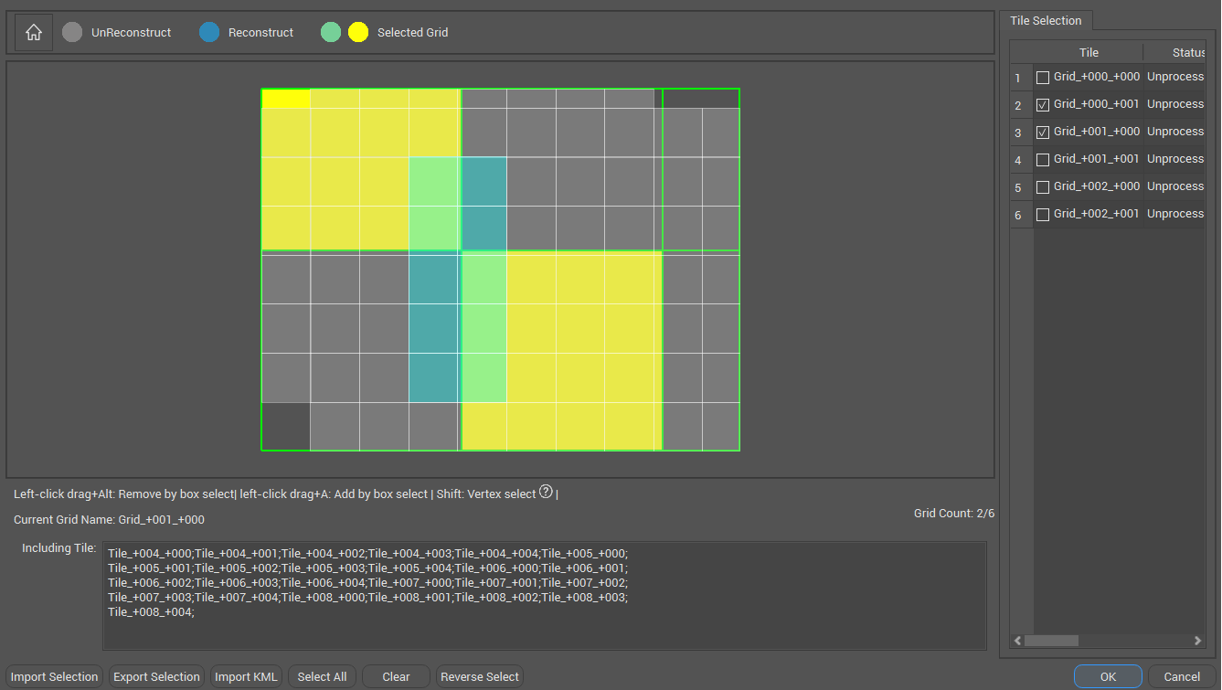
Click on **Select Grids** to selectively model parts of the entire interior of the area.

<figure><img src="/files/ZczGBvBe0pQ29MKXMhz5" alt=""><figcaption><p>Select Grids</p></figcaption></figure>

After all the settings are done, you can click **OK** to submit the production and enter the reconstruction calculation.

<figure><img src="/files/MPMZDGHtvkDfZoESVs2N" alt=""><figcaption><p>Production Running</p></figcaption></figure>

After successful tile reconstruction, users can view 2D products with one click in Get3D Viewer (v4.1.0 or later) when both DOM and DSM outputs are available.

<figure><img src="/files/b7aSDN7l8T4FDdRl2w47" alt=""><figcaption><p>Open with Get3D Viewer</p></figcaption></figure>


# Edit Control Points

This chapter introduces how to edit control points and complete the absolute orientation (AT).

If the product generated by only inputting the photo positioning data does not meet the absolute accuracy requirement, control points should be added after the relative orientation to achieve absolute orientation and improve the absolute accuracy of the product.

## Working Interface

Click **Edit GCP** to open the control point editing interface, as shown in the figure below:

<figure><img src="/files/Omi5QLETDNPtfjgwsQ4J" alt=""><figcaption><p>Edit Control Points Interface</p></figcaption></figure>

The interface is divided into four parts: Control Point Information, Marking Point Information,  View Panel and Photos Preview Panel

The control point information bar displays the point information of the imported control point, and the marking point information bar displays the marking point information of each control point. The table header information is shown in the table, as shown below.

<figure><img src="/files/MLUku8qSCLYCozeBhU47" alt=""><figcaption><p>Control Point Information</p></figcaption></figure>

The view panel includes the Block View, 3D View, and Control Points Record.

Block View displays a 2D view of the photos and control points within the block. It is primarily used for selecting, locking, and unlocking control points.

<figure><img src="/files/WdeQTdqtmwqEk7uYTtEt" alt=""><figcaption><p>Block View</p></figcaption></figure>

3D View displays the spatial positions of control points, point clouds, and photos.

<figure><img src="/files/q896f67NnMToeQnskSt6" alt=""><figcaption><p>3D View</p></figcaption></figure>

Control Points Record shows the point records collected in the field, which are used to determine the actual location corresponding to the marked points. Users can refer to the point record to perform marking operations.

<figure><img src="/files/hceTIAIEFPwITB4ZXhrT" alt=""><figcaption><p>Control Points Record</p></figcaption></figure>

Photos preview panel shows photos to be marked and marking tools.

<figure><img src="/files/MFkbBnG7BquE07BfBgAg" alt=""><figcaption><p>Photos Preview</p></figcaption></figure>

<figure><img src="/files/IXAQuY7iLcMGiEInCdON" alt=""><figcaption><p>Button Table</p></figcaption></figure>

## Workflow

### **Import Control Points**

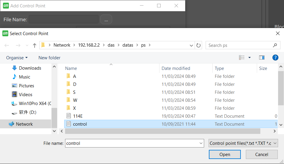
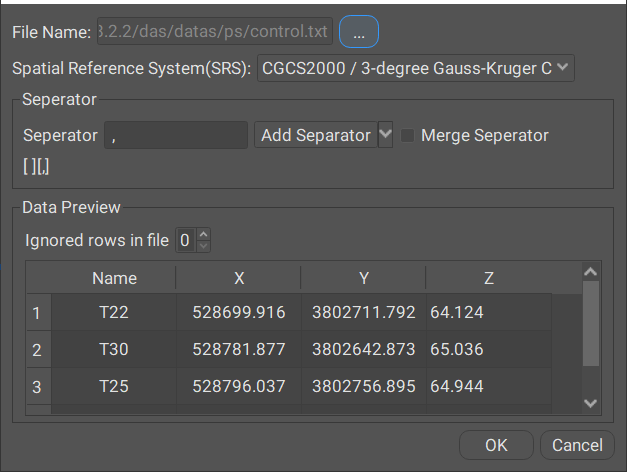
Click **Import**, select the spatial reference corresponding to the control point file, select the separator, set the name, X, Y, Z, and click **OK** to import the control points.

<figure><img src="/files/g6uHy5CMiQQcxxcMhGcX" alt=""><figcaption><p>Import Control Points</p></figcaption></figure>

### **Mark GCPs**

Get3D Mapper supports manual marking points and intelligent marking points.

<mark style="color:yellow;background-color:yellow;">**Manual Marking:**</mark>

1\) Select Control Points:

In the Control Point Information Panel or Block View, select the control point to mark.

Photos containing the selected control point will appear in the Photo Preview Panel. By default, photos with the point centered are displayed first, filling the panel in a tiled layout.

2\) Adjust Photo Display:

The number of photos displayed per page can be adjusted. For example, if 4 photos are set per page, they will be displayed in an appropriate size.

3\) Mark Control Points:

Photo names are highlighted with a yellow border. Selected photos are marked with a blue border.

Hold the **Shift** key and **left-click** to mark the point. The marking position is confirmed based on field data collection.

After marking, the photo name changes to a green border, and marking details appear in the Marking Information Panel.

Once two photos are marked, a red prediction box will appear in subsequent photos, guiding the marking process. Press **D** to switch to the next page.

{% hint style="warning" %}
For optimal accuracy, it is recommended to mark approximately **30** photos per control point.&#x20;
{% endhint %}

<figure><img src="/files/ugoXCoJi5a1yxVoFnTcI" alt=""><figcaption><p>Marking Points</p></figcaption></figure>

<figure><img src="/files/AMuNI0NWNGM7UFfD6Rrh" alt=""><figcaption><p>After Marking</p></figcaption></figure>

<mark style="color:yellow;background-color:yellow;">**Intelligent Marking:**</mark>

1\) Initial Marking:

Mark two photos manually for the control point.

2\) Intelligent Recognition:

Click **Intelligent Recognition**, and the software predicts the corresponding positions in other photos.

Photos with successful predictions are marked with a green border. Those without predictions remain with a yellow border and require manual marking.

<figure><img src="/files/WBnqC54liVMzq57S8vgo" alt=""><figcaption><p>Intelligent Recognition</p></figcaption></figure>

3\) Check and Confirm:

Verify the results on the current page. Adjust positions as needed.

Click **Confirm Position** to save the markings to the Marking Information Panel.

After confirming positions, the predicted points will change to red.

<figure><img src="/files/ym2qJ7wdBJFXJMQtKBwf" alt=""><figcaption><p>Before Confirming</p></figcaption></figure>

<figure><img src="/files/gf9iqyyqZTtW0ClOSVbd" alt=""><figcaption><p>After Confirming</p></figcaption></figure>

4\) Repeat for Remaining Photos:

Navigate to the next page and repeat the steps until the required number of photos is marked with satisfactory precision.

Some of the common shortcuts for Mark GCPs is shown:

<figure><img src="/files/H0V6fHHeikIbzmUr2VKD" alt="" width="563"><figcaption><p>Shortcut</p></figcaption></figure>

### **Save Marking Results**

After completing the marking, close the marking panel and save the edits to the block file.

### Submit AT

After editing control points, click **Submit AT** and  submit the absolute orientation. After AT processing( absolute orientation), continue submitting 3D reconstruction according to the workflow.

<figure><img src="/files/7rxK4bgQMIOFiKTon0Dx" alt=""><figcaption><p>Absolute Orientation</p></figcaption></figure>

## AT Constraint

**Usage:**\
For AT results generated from non-georeferenced data (relative orientation), a new *Constraints* tool is available under the Edit Control Points module.\
This allows you to add geometric or spatial constraints by linking control points to improve accuracy, correct deviations, or ensure geometric consistency.\
Create tie points by manually marking the same feature on multiple photos.

**Steps:**

1. Mark at least 2 tie points.
2. Click *Add Constraints* to open the Constraints interface.

<figure><img src="/files/wMwTc6Mqn7PrxYuDcLfi" alt=""><figcaption></figcaption></figure>

3. Select the constraint type.

<figure><img src="/files/0ghc3CNq6m7gtitjelmH" alt=""><figcaption></figcaption></figure>

Supported types:

* **Scale Constraint:** Define the distance between two tie points to correct the model scale (e.g., building width, paint mark spacing).

<figure><img src="/files/alx07kT11oteCWkblAWj" alt=""><figcaption></figcaption></figure>

* **Planar Constraint:** Force three tie points to lie on the same plane and align with a chosen coordinate axis plane (e.g., level ground or vertical wall).

<figure><img src="/files/1hjngexl9q4kcHD6lAvg" alt=""><figcaption></figcaption></figure>

* **Orientation Constraint:** Align the direction between two connection points parallel to a specified axis.

<figure><img src="/files/Bo9xBJMxZc7C6FC2Z9L1" alt=""><figcaption></figcaption></figure>

4. Set parameters, and click *Apply* to preview. Click *Reset* to revert to the original AT result.

When closing, you will be prompted *“Save AT?”* Click *Yes* to apply the constraint to the block, or *No* to discard changes.


# Edit Control Points\_V7.1.5

This chapter introduces how to edit control points and complete the absolute orientation (AT).

If the product generated by only inputting the photo positioning data does not meet the absolute accuracy requirement, control points should be added after the relative orientation to achieve absolute orientation and improve the absolute accuracy of the product.

## Working Interface

Click **Edit GCP** to open the control point editing interface, as shown in the figure below:

<figure><img src="/files/Omi5QLETDNPtfjgwsQ4J" alt=""><figcaption><p>Edit Control Points Interface</p></figcaption></figure>

The interface is divided into four parts: Control Point Information, Marking Point Information,  View Panel and Photos Preview Panel

The control point information bar displays the point information of the imported control point, and the marking point information bar displays the marking point information of each control point. The table header information is shown in the table, as shown below.

<figure><img src="/files/MLUku8qSCLYCozeBhU47" alt=""><figcaption><p>Control Point Information</p></figcaption></figure>

The view panel includes the Block View, 3D View, and Control Points Record.

Block View displays a 2D view of the photos and control points within the block. It is primarily used for selecting, locking, and unlocking control points.

<figure><img src="/files/WdeQTdqtmwqEk7uYTtEt" alt=""><figcaption><p>Block View</p></figcaption></figure>

3D View displays the spatial positions of control points, point clouds, and photos.

<figure><img src="/files/q896f67NnMToeQnskSt6" alt=""><figcaption><p>3D View</p></figcaption></figure>

Control Points Record shows the point records collected in the field, which are used to determine the actual location corresponding to the marked points. Users can refer to the point record to perform marking operations.

<figure><img src="/files/hceTIAIEFPwITB4ZXhrT" alt=""><figcaption><p>Control Points Record</p></figcaption></figure>

Photos preview panel shows photos to be marked and marking tools.

<figure><img src="/files/MFkbBnG7BquE07BfBgAg" alt=""><figcaption><p>Photos Preview</p></figcaption></figure>

<figure><img src="/files/IXAQuY7iLcMGiEInCdON" alt=""><figcaption><p>Button Table</p></figcaption></figure>

## Workflow

### **Import Control Points**

Click **Import**, select the spatial reference corresponding to the control point file, select the separator, set the name, X, Y, Z, and click **OK** to import the control points.

<figure><img src="/files/g6uHy5CMiQQcxxcMhGcX" alt=""><figcaption><p>Import Control Points</p></figcaption></figure>

### **Mark GCPs**

Get3D Mapper supports manual marking points and intelligent marking points.

<mark style="color:yellow;background-color:yellow;">**Manual Marking:**</mark>

1\) Select Control Points:

In the Control Point Information Panel or Block View, select the control point to mark.

Photos containing the selected control point will appear in the Photo Preview Panel. By default, photos with the point centered are displayed first, filling the panel in a tiled layout.

2\) Adjust Photo Display:

The number of photos displayed per page can be adjusted. For example, if 4 photos are set per page, they will be displayed in an appropriate size.

3\) Mark Control Points:

Photo names are highlighted with a yellow border. Selected photos are marked with a blue border.

Hold the **Shift** key and **left-click** to mark the point. The marking position is confirmed based on field data collection.

After marking, the photo name changes to a green border, and marking details appear in the Marking Information Panel.

Once two photos are marked, a red prediction box will appear in subsequent photos, guiding the marking process. Press **D** to switch to the next page.

{% hint style="warning" %}
For optimal accuracy, it is recommended to mark approximately **30** photos per control point.&#x20;
{% endhint %}

<figure><img src="/files/ugoXCoJi5a1yxVoFnTcI" alt=""><figcaption><p>Marking Points</p></figcaption></figure>

<figure><img src="/files/AMuNI0NWNGM7UFfD6Rrh" alt=""><figcaption><p>After Marking</p></figcaption></figure>

<mark style="color:yellow;background-color:yellow;">**Intelligent Marking:**</mark>

1\) Initial Marking:

Mark two photos manually for the control point.

2\) Intelligent Recognition:

Click **Intelligent Recognition**, and the software predicts the corresponding positions in other photos.

Photos with successful predictions are marked with a green border. Those without predictions remain with a yellow border and require manual marking.

<figure><img src="/files/WBnqC54liVMzq57S8vgo" alt=""><figcaption><p>Intelligent Recognition</p></figcaption></figure>

3\) Check and Confirm:

Verify the results on the current page. Adjust positions as needed.

Click **Confirm Position** to save the markings to the Marking Information Panel.

After confirming positions, the predicted points will change to red.

<figure><img src="/files/ym2qJ7wdBJFXJMQtKBwf" alt=""><figcaption><p>Before Confirming</p></figcaption></figure>

<figure><img src="/files/gf9iqyyqZTtW0ClOSVbd" alt=""><figcaption><p>After Confirming</p></figcaption></figure>

4\) Repeat for Remaining Photos:

Navigate to the next page and repeat the steps until the required number of photos is marked with satisfactory precision.

Some of the common shortcuts for Mark GCPs is shown:

<figure><img src="/files/H0V6fHHeikIbzmUr2VKD" alt="" width="563"><figcaption><p>Shortcut</p></figcaption></figure>

### **Save Marking Results**

After completing the marking, close the marking panel and save the edits to the block file.

### Submit AT

After editing control points, click **Submit AT** and  submit the absolute orientation. After AT processing( absolute orientation), continue submitting 3D reconstruction according to the workflow.

<figure><img src="/files/7rxK4bgQMIOFiKTon0Dx" alt=""><figcaption><p>Absolute Orientation</p></figcaption></figure>

## AT Constraint

**Usage:**\
For AT results generated from non-georeferenced data (relative orientation), a new *Constraints* tool is available under the Edit Control Points module.\
This allows you to add geometric or spatial constraints by linking control points to improve accuracy, correct deviations, or ensure geometric consistency.\
Create tie points by manually marking the same feature on multiple photos.

**Steps:**

1. Mark at least 2 tie points.
2. Click *Add Constraints* to open the Constraints interface.

<figure><img src="/files/wMwTc6Mqn7PrxYuDcLfi" alt=""><figcaption></figcaption></figure>

3. Select the constraint type.

<figure><img src="/files/0ghc3CNq6m7gtitjelmH" alt=""><figcaption></figcaption></figure>

Supported types:

* **Scale Constraint:** Define the distance between two tie points to correct the model scale (e.g., building width, paint mark spacing).

<figure><img src="/files/alx07kT11oteCWkblAWj" alt=""><figcaption></figcaption></figure>

* **Planar Constraint:** Force three tie points to lie on the same plane and align with a chosen coordinate axis plane (e.g., level ground or vertical wall).

<figure><img src="/files/1hjngexl9q4kcHD6lAvg" alt=""><figcaption></figcaption></figure>

* **Orientation Constraint:** Align the direction between two connection points parallel to a specified axis.

<figure><img src="/files/Bo9xBJMxZc7C6FC2Z9L1" alt=""><figcaption></figcaption></figure>

4. Set parameters, and click *Apply* to preview. Click *Reset* to revert to the original AT result.

When closing, you will be prompted *“Save AT?”* Click *Yes* to apply the constraint to the block, or *No* to discard changes.


# Point Cloud Modeling

In addition to image data, Get3D Mapper also supports point cloud modeling and point cloud-image fusion modeling.

## **Point Cloud Modeling**

### **Add Mobile Laser Scanning**

Get3D Mapper supports the addition of laser point cloud and track line data collected by mobile laser equipment. The software supports laser point cloud modeling alone and laser point cloud fusion modeling with photos.

Support vehicle-mounted, airborne, backpack, and handheld laser point clouds. Laser point cloud supported formats: \*.las, \*.ptx, \*.pts, \*.e57. Trajectory line supported formats: \*.txt, \*csv.

**1) Open the Add Mobile Laser Scanning interface**

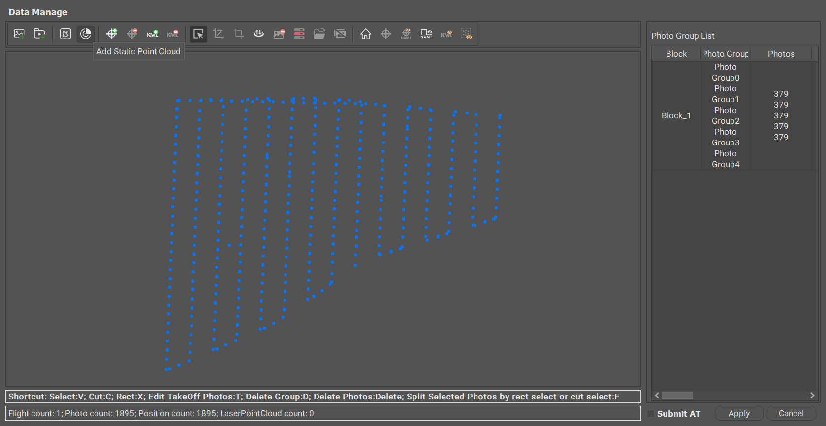
<figure><img src="/files/P1Uf1r8nUlsAQ956xlIT" alt=""><figcaption><p>Data Prepare Interface</p></figcaption></figure>

<figure><img src="/files/3BqT5v4P3lmMdaMETdbY" alt=""><figcaption><p>Add Mobile Laser Scanning Interface</p></figcaption></figure>

<figure><img src="/files/gJ3mEF7pBeJSxlO2zYre" alt=""><figcaption><p>Add Mobile Scan Overview</p></figcaption></figure>

**2) Setting up the laser point cloud spatial reference**

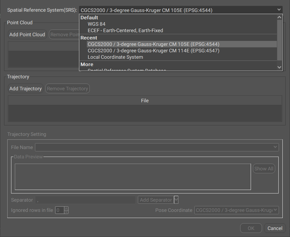
<figure><img src="/files/G26bU6gCQWcFnmc8rvTw" alt=""><figcaption><p>Set Coordinate System for Point Cloud</p></figcaption></figure>

**3) Add Point Cloud Data**

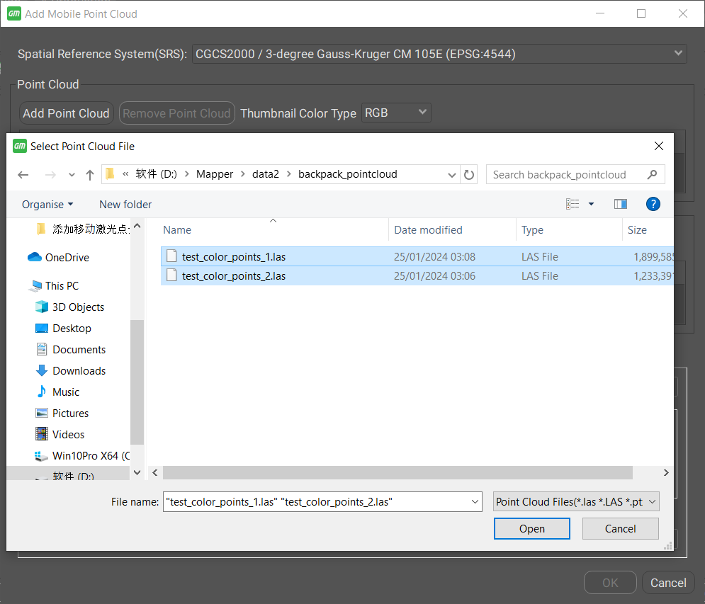
<figure><img src="/files/7IdHY3s6QakgP13IXSQk" alt=""><figcaption><p>Add Point Cloud File</p></figcaption></figure>

**4) Add Trajectory Files**

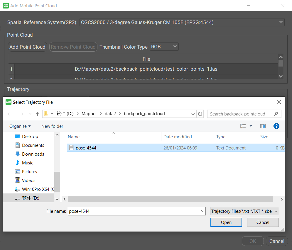
<figure><img src="/files/P9H028iWeFLeQQi3Gzfl" alt=""><figcaption><p>Add Trajectory Files</p></figcaption></figure>

**5) Define the trajectory**

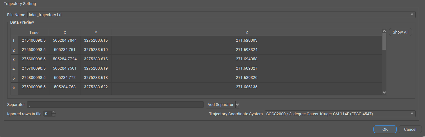
Set the spatial reference of the track line, the separator, and the actual meaning corresponding to each column ("GPS time, longitude, latitude, elevation" or "GPS time, east coordinate, north coordinate, elevation").

<figure><img src="/files/20UpFSRDzGGbf2GuAkrb" alt=""><figcaption><p>Define the Trajectory</p></figcaption></figure>

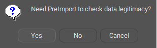
&#x20;**6) Enquiry**

Whether you need to check for data matching.

<figure><img src="/files/XiS4EGO3xL4rsm4kpZYW" alt=""><figcaption></figcaption></figure>

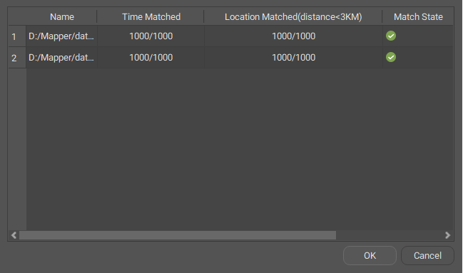
**7) Check the matching results**

Laser point cloud check contains laser point position and track line position matching; laser point cloud time and track line time matching. And display the matching status.

<figure><img src="/files/TgsUIgmhFbuz0681Yrpm" alt=""><figcaption><p>Point Cloud Check</p></figcaption></figure>

**8) Apply point cloud**

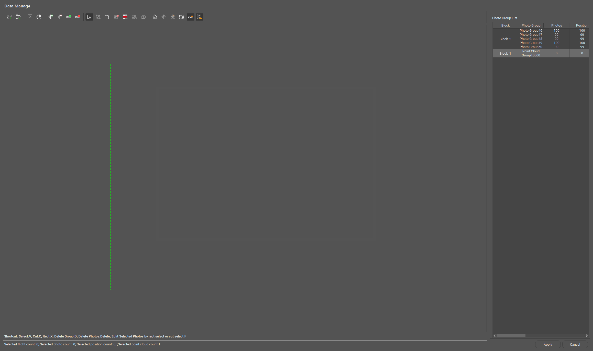
After importing point cloud, click **Apply** to generate a new block.

<figure><img src="/files/fFZYuuiKYLo78CWNG1Vd" alt=""><figcaption><p>Apply Point Cloud</p></figcaption></figure>

### **Add Terrestrial Laser Scanning**

Get3D Mapper supports adding laser point cloud and center data collected by a stationary laser equipment. The software can support laser point cloud modeling alone and laser point cloud and photo fusion modeling. The following formats are supported: \*.las, \*.ptx, \*.pts, and \*.e57. The station center supports manual input or import of \*.txt format files.

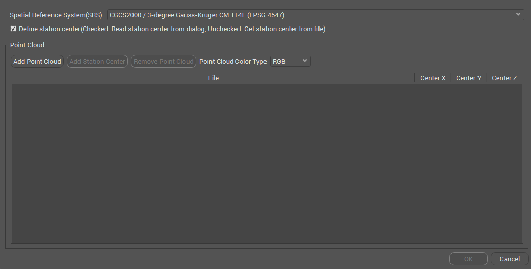
<figure><img src="/files/KMUEBUniBDjWzSBIsKPq" alt=""><figcaption><p>Add Terrestrial Laser Scanning</p></figcaption></figure>

<figure><img src="/files/hvRBL4S1yVAd7ilVwkdb" alt=""><figcaption><p>Add Terrestrial Laser Scanning Interface</p></figcaption></figure>

<figure><img src="/files/AcNACf8MkhG38CHJUf5F" alt="" width="563"><figcaption><p>Add Static Scan Overview</p></figcaption></figure>

**1) Select the point cloud coordinate system**

<figure><img src="/files/bHlciTRTbsYkRFG36ke4" alt=""><figcaption></figcaption></figure>

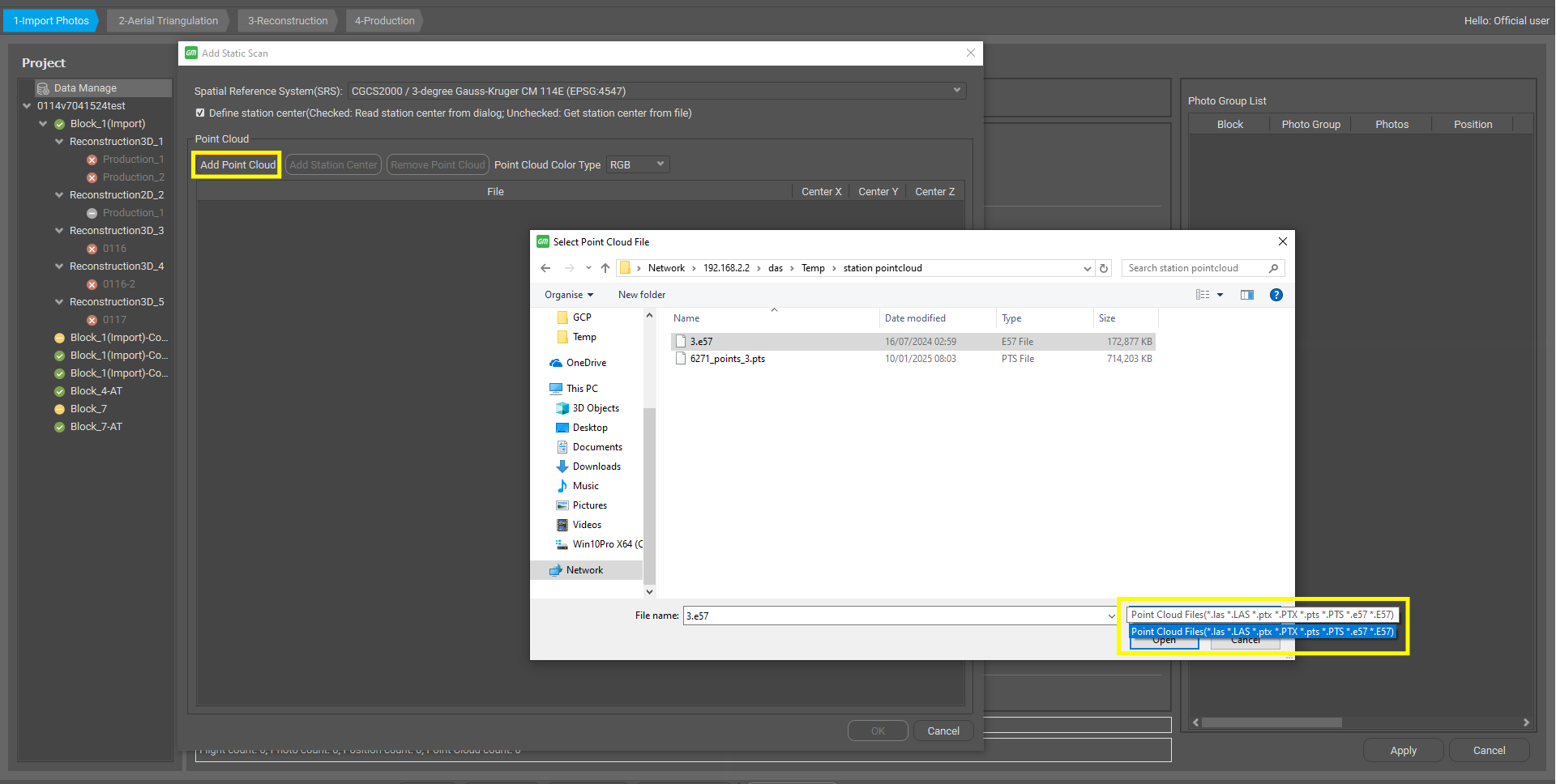
**2) Add Point Cloud**

<figure><img src="/files/7KXP7Yke51gT11Kd9A9M" alt=""><figcaption></figcaption></figure>

**3) Add station Center**

There are two ways to add station center coordinates:

One is to manually add station center coordinates on the right side of the point cloud list.

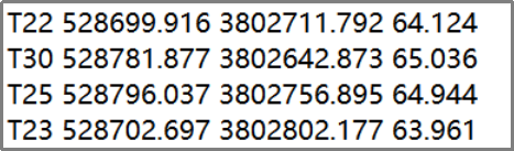
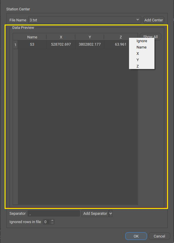
The other is to click **Add Station Center**, import the center of the station coordinates file. File samples such as the figure below, including the point cloud name, x, y, z arrangement, separated by a space in the middle:

<figure><img src="/files/zp2x9UTdHSv6yIXUsuZC" alt=""><figcaption><p>Station Center File</p></figcaption></figure>

<figure><img src="/files/KVKZK6px7vnb220lRWWN" alt=""><figcaption><p>Add Station Center File</p></figcaption></figure>

<figure><img src="/files/QY7CZUjdNZQeORU0MLpT" alt=""><figcaption><p>Set Station Center and Apply</p></figcaption></figure>

If there is no station center coordinates, the software can automatically calculate, uncheck the Define station center.

**4) Apply point cloud**

After importing point cloud, click **OK** to generate a new block.

<figure><img src="/files/A9JA5Hg5IG1SF8aGGfkS" alt=""><figcaption></figcaption></figure>

### Process Point Cloud

In the point cloud block, navigate to the **Point Cloud** panel and click **Process** to cut the point cloud.

<figure><img src="/files/K1lbZiRYmN4knZgNFZ4K" alt=""><figcaption><p>Process Point Cloud</p></figcaption></figure>

After processing, you can view and check the point cloud in the 3D view.

If point cloud checked, then continue create a new 3D reconstruction according to the workflow.

## Point Cloud-Image Fusion Modeling

Get3D Mapper supports importing laser point cloud data and fusing it with image data for modeling. Multi-source data fusion modeling can solve the texture distortion, feature voids and other defects in the 3D modeling process.

Image data is first imported for aerial triangulation (Relative Orientation).

For data containing control points, Absolute Orientation should be completed before importing the laser data for fusion modeling.

After AT, open the Point Cloud panel, select the point cloud type, and add the data (e.g., mobile LiDAR).

<figure><img src="/files/hEl6oPmiThqH6C8VvMzU" alt=""><figcaption><p>Point Cloud Panel</p></figcaption></figure>

Imports laser data: The laser data consists of .las point cloud files, and .txt point cloud trajectory line files.

Click **Add Mobile Point Cloud**, select the correct coordinate system, import the point cloud file in ".las" format, and the trajectory line file in ".txt" format.

<figure><img src="/files/Z7I4hRKmLyPpaxgp2BZk" alt=""><figcaption><p>Add Point Cloud</p></figcaption></figure>

<figure><img src="/files/P9H028iWeFLeQQi3Gzfl" alt=""><figcaption><p>Add Trajectory</p></figcaption></figure>

**Note: The correct coordinate system should be selected for both files.**

Where the trajectory line file needs to correspond to: Time, X, Y, Z

<figure><img src="/files/20UpFSRDzGGbf2GuAkrb" alt=""><figcaption><p>Set Parameters</p></figcaption></figure>

Click **OK** and the software automatically matches the point cloud data with the track line. The two correspond to each other and the submission is successful.

<figure><img src="/files/xugG2gLeCVMwgzn6tf2W" alt=""><figcaption><p>Check Point Cloud</p></figcaption></figure>

Click **Process** in Point Cloud Process to slice the tiles. Once you have finished slicing the tiles, you can view both the point cloud trace lines and the image photo shelf in the 3D view.

<figure><img src="/files/YHWSxE5lyhczArJ37yvV" alt=""><figcaption><p>Process Point Cloud</p></figcaption></figure>

<figure><img src="/files/qLMl2stzccy8QrcQMe9Q" alt=""><figcaption><p>Process Point Cloud Finished</p></figcaption></figure>

Right click to submit Reconstruction for multi-source data fusion modeling.

<figure><img src="/files/XJ5qlxVxSTqHBjT1QcXE" alt=""><figcaption><p>New 3D Reconstruction</p></figcaption></figure>

Tutorial video: <https://www.youtube.com/watch?v=FRhEHu-5vNA>


# AT Setting Instruction

**Objective of Aerial Triangulation:**

**Aerial Triangulation** (AT) aims to use the camera's imaging model to recover the camera's position and orientation during capture.

**Relative Orientation** utilizes the camera's initial internal orientation elements and the relationship between correspondence points to recover the camera’s position and orientation in the relative coordinate system, along with camera’s internal parameters, distortion, and object space point coordinate.

**Absolute Orientation** converts the relative local coordinate system into the absolute world coordinate system using results from the relative orientation and ground control points.

## 1 Aerial Triangulation Setting Interface

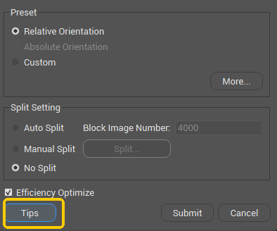
<figure><img src="/files/af2lh2sLBi1uwCKTCeDg" alt=""><figcaption></figcaption></figure>

### 1.1 Preset

**Relative Orientation:** Input photos (POS optional), recover the photo's position and orientation, and generate a sparse point cloud.

**Absolute Orientation:** Add control points to the relative AT results, perform absolute orientation, and improve the absolute accuracy of AT.

**Custom:** Custom AT settings for specific AT scenarios.

**More:** Additional AT settings. The interface simplifies default operations and opens up more AT parameters, allowing users to adjust settings to better suit the current scenario when processing data.

<figure><img src="/files/fXkmK1mYZcfDf9jogFaI" alt=""><figcaption></figcaption></figure>

<figure><img src="/files/xhsoN2lwENRaIzQ2hJDH" alt=""><figcaption></figcaption></figure>

Both **Bundle Constraint** and **Positioning Method** can be selected simultaneously. The settings in the Positioning Method are used for rigid registration, while the settings in the Bundle Constraint are used for constraint adjustment.

### 1.2 Split Setting

#### **1.2.1 Relative Orientation Split Setting**

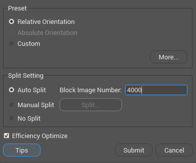
<figure><img src="/files/1MkMuSBLqM3a6YFYYgs8" alt=""><figcaption></figcaption></figure>

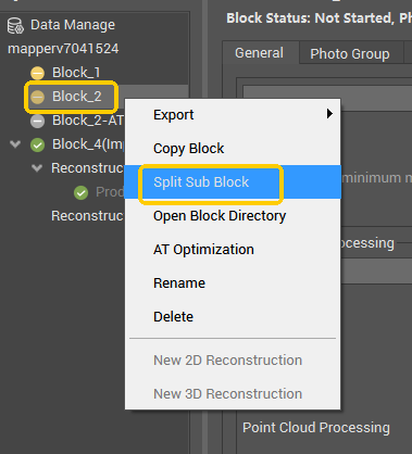
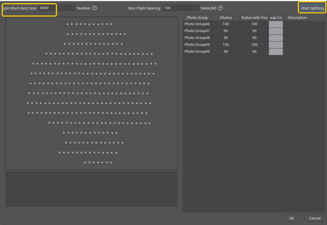
**Auto Split** and **Manual Split** processing in the relative AT bundle phase utilizes a multi-machine parallel processing strategy, improving the computational efficiency when using cluster for large-scale AT. For cases with more than 8,000 photos, it is recommended to divide into sub-blocks.

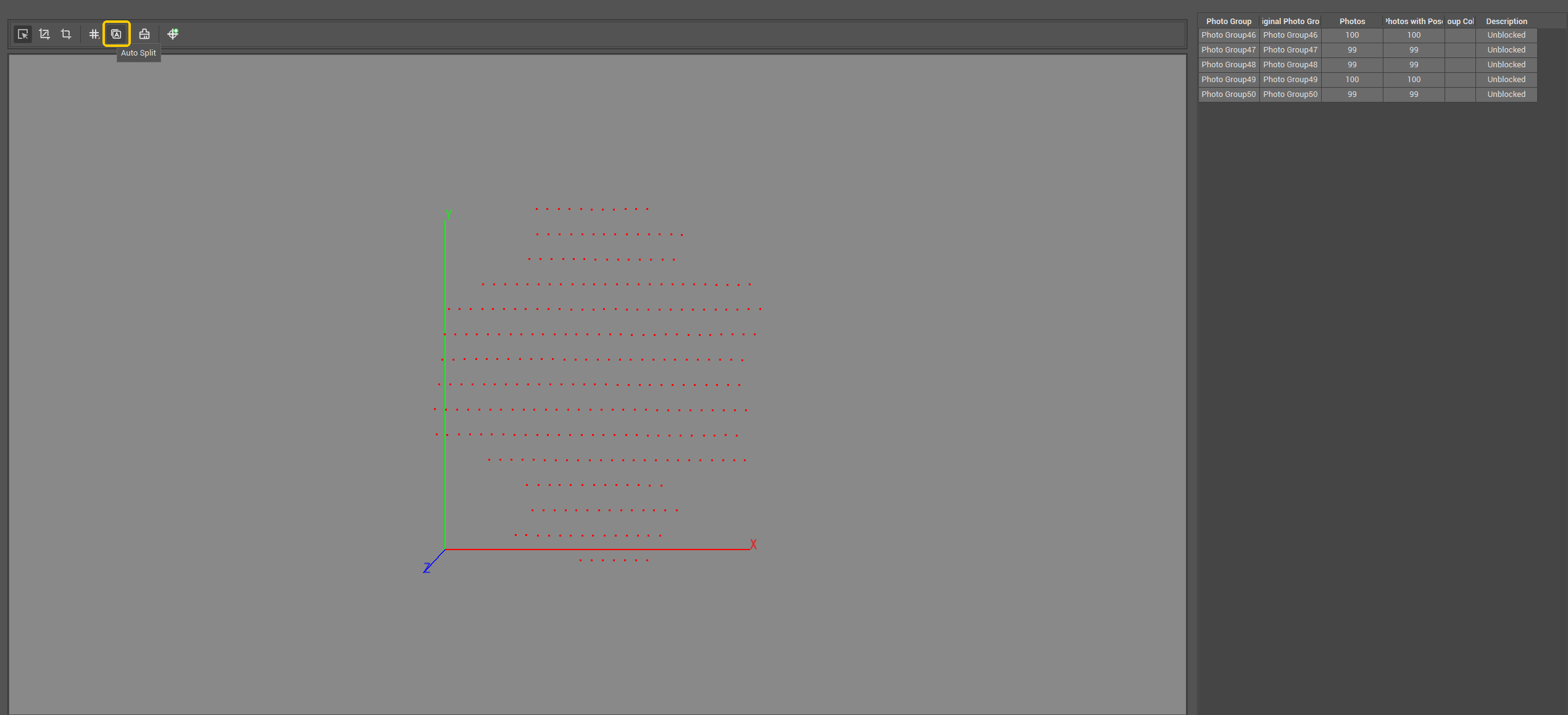
**Auto Split:** Each photo has position information. Photos acquired along regular flight lines are automatically divided into sub-blocks based on the set number of photos per sub-block.

**Manual Split:** Used when some POS data is missing or unavailable, dividing photos into sub-blocks based on photo groups.

**No Split:** Recommended when the total photo count is less than 8,000.

The AT process involves moving from one stage to the next after completing the previous task. Multi-task stages can run in parallel on multiple machines, while single-task stages are processed on a single machine. (It is normal for some engines waiting during the AT process.)

<figure><img src="/files/QsBW8mnoyoYxyb54i7Xt" alt=""><figcaption></figcaption></figure>

#### **1.2.2 Absolute Orientation Split Setting**

<figure><img src="/files/NTDgysPgyHx0yHbhXsEt" alt=""><figcaption></figcaption></figure>

**Auto Split** processing in the absolute AT bundle phase utilizes a multi-machine parallel processing strategy, improving the computational efficiency when using cluster for large-scale AT. For cases with more than 50,000 photos, it is recommended to divide into sub-blocks.

**Auto Split:** Significantly improves Absolute AT speed. If the number of control points is less than 10, it is not recommended to split block. The default setting of 50,000 images per block is recommended. Setting it too small may result in sub-blocks with no control points.

**No Split:** A single task is generated and can only be processed on one machine.

The AT process involves moving from one stage to the next after completing the previous task. Multi-task stages can run in parallel on multiple machines, while single-task stages are processed on a single machine. (It is normal for some engines waiting during the AT process.)

<figure><img src="/files/oIktrNVuqQ3VbEUTCFRa" alt=""><figcaption></figcaption></figure>

### **1.3 Efficiency Optimization**

It is recommended to select Efficiency Optimization for oblique image data. Deselecting Efficiency Optimization requires more memory and longer computation time. A computer with 64GB of memory can process up to 100,000 images.

## 2 Relative Orientation

### 2.1 Oblique Image

For oblique data, it is recommended to submit with the default parameters. For the city scene, it's recommended to select Efficiency Optimization

<figure><img src="/files/af2lh2sLBi1uwCKTCeDg" alt=""><figcaption></figcaption></figure>

### 2.2 Orthophoto

#### 2.2.3 General Orthophoto Image

Recommended parameters for general orthophoto scenes.

* [ ] Efficiency Optimize

Image Paris Filter Level--**Medium**

* [x] Pose Metadata

{% hint style="info" %}
It is recommended to use for high-accuracy GPS and fill in the camera accuracy. Low-accuracy GPS as bundle constraint input will affect the overall accuracy of aerial triangulation.
{% endhint %}

<div><figure><img src="/files/af2lh2sLBi1uwCKTCeDg" alt=""><figcaption></figcaption></figure> <figure><img src="/files/KA0PKjpgXlIxk6BQKJAU" alt=""><figcaption></figcaption></figure></div>

Default parameters for AT, the results are distorted.

<div><figure><img src="/files/J6WFtuaifREY9AxBRe3w" alt=""><figcaption></figcaption></figure> <figure><img src="/files/bGpVmwe8neZ5KPfxJrkU" alt=""><figcaption></figcaption></figure></div>

<div><figure><img src="/files/q2kanhyBt3FnCkU4NDGr" alt=""><figcaption></figcaption></figure> <figure><img src="/files/qoWxcy4FZneUbkduqWob" alt=""><figcaption></figcaption></figure></div>

Recommended parameters for AT, the results are normal.

<div><figure><img src="/files/19yILruIaNwRX7rqWHGL" alt=""><figcaption></figcaption></figure> <figure><img src="/files/SzPMTE5wCLbe1zGo0LNY" alt=""><figcaption></figcaption></figure></div>

<div><figure><img src="/files/mFItyOUuNzs7L4WydfJj" alt=""><figcaption></figcaption></figure> <figure><img src="/files/tNPahTHK0eUsjKmE7mu3" alt=""><figcaption></figcaption></figure></div>

#### 2.2.2 Weak Texture Orthophoto Image

Recommended parameters for weak texture orthophoto scenes.

* [ ] Efficiency Optimize

Keypoints Density--**High**

Image Paris Filter Level--**Medium**

* [x] Pose Metadata

{% hint style="info" %}
It is recommended to use for high-accuracy GPS and fill in the camera accuracy. Low-accuracy GPS as bundle constraint input will affect the overall accuracy of aerial triangulation.
{% endhint %}

<div><figure><img src="/files/FhRHxbqzBWIXQ8csF2Yj" alt=""><figcaption></figcaption></figure> <figure><img src="/files/7M0kUj7mFLOofF9oYNZm" alt=""><figcaption></figcaption></figure></div>

Default parameters for AT, the calibrated photo rate is low (left side). Recommended parameters for AT, all photos calibrated (right side).

<div><figure><img src="/files/WVdwKxYVDQr3OkaQiUPe" alt=""><figcaption></figcaption></figure> <figure><img src="/files/TOfkUiVrdlGFmV517UEA" alt=""><figcaption></figcaption></figure></div>

<div><figure><img src="/files/if9jSfDlfgjAcYLepwBs" alt=""><figcaption></figcaption></figure> <figure><img src="/files/h0u6H4EMOPKEG7lm8MgL" alt=""><figcaption></figcaption></figure></div>

#### 2.2.3 Orthophoto with High POS Accuracy

* [ ] Efficiency Optimization

Keypoints Density--**High**

Image Paris Filter Level--**Low**

Facal Length--**Keep**

* [x] Pose Metadata

{% hint style="info" %}
It is recommended to use for high-accuracy GPS and fill in the camera accuracy. Low-accuracy GPS as bundle constraint input will affect the overall accuracy of aerial triangulation.
{% endhint %}

<div><figure><img src="/files/vX03wtDh0csfI33bdQun" alt=""><figcaption></figcaption></figure> <figure><img src="/files/erHNpKAKYDjOI8fxInFf" alt=""><figcaption></figcaption></figure></div>

### 2.3 Road

#### **2.3.1** Single-Camera Road Orbit Route

* [ ] &#x20;Efficiency Optimization

Search Range--**Diameter of one circle of the flight**

Image Paris Filter Level--**Medium**

* [x] Pose Metadata

<div><figure><img src="/files/1fCHROF3t9WQWcI9OpJ6" alt=""><figcaption></figcaption></figure> <figure><img src="/files/r3IkyZ9xwlOcjLf2pzMb" alt=""><figcaption></figcaption></figure></div>

Default parameters for AT, some images lost (blue area).

<div><figure><img src="/files/Hp4xrnyTMEn5691NvNDN" alt=""><figcaption></figcaption></figure> <figure><img src="/files/XkKtfAmOBRMS97yXVk3H" alt=""><figcaption></figcaption></figure></div>

Only select Pose Metadata for AT, the number of lost photos is reduced.

<div><figure><img src="/files/hex7yLFDtIbNeH0pd8KM" alt=""><figcaption></figcaption></figure> <figure><img src="/files/8rlmbQCHl39jsbFlP38k" alt=""><figcaption></figcaption></figure></div>

Recommended parameters for AT, all images are in net.

<div><figure><img src="/files/23rb3zajDGWC2NYSQu6W" alt=""><figcaption></figcaption></figure> <figure><img src="/files/emD00n93hRXZE3tK6IY7" alt=""><figcaption></figcaption></figure></div>

#### **2.3.2** Oblique Five-Camera Road Flight Route

Recommended parameters for 5-lens rule flight.

* [x] Pose Metadata

<div><figure><img src="/files/2dpOCfDhW1FR0OPA6vDz" alt=""><figcaption></figcaption></figure> <figure><img src="/files/kqsfgMdA8GGfJA2oni19" alt=""><figcaption></figcaption></figure></div>

### 2.4 POS High Accuracy

#### **2.4.1 Before Submitting AT**

In the relative orientation stage, select **Pose Metadata** to improve AT absolute accuracy.

* [x] Pose Metadata

<div><figure><img src="/files/2dpOCfDhW1FR0OPA6vDz" alt=""><figcaption></figcaption></figure> <figure><img src="/files/BVLODqhBXjrQbWZBHTnc" alt=""><figcaption></figcaption></figure></div>

**2.4.2 Resubmit after Relative Orientation**

AT absolute accuracy can be improved by selecting Pose Metadata and applying Bundle Constraints through Custom parameter settings. The parameter settings are as follows:

◉ Custom

◉ No Split

&#x20;Photo Selection--**Photos in Net**

Tie Points--**Keep**

* [x] Pose Metadata

<div><figure><img src="/files/YxVfPA8dmjYx9WYEdhol" alt=""><figcaption></figcaption></figure> <figure><img src="/files/M7L6c0gypwCYP7VCYXGw" alt=""><figcaption></figcaption></figure></div>

### 2.5 Close Range

Recommended for close-range capture. Do not split sub-blocks. Try selecting parameters to adjust different combinations.

<div><figure><img src="/files/1nfIpXAseomuDSNuTOeY" alt=""><figcaption></figcaption></figure> <figure><img src="/files/fcuSeIRbuCUUOs3lKieX" alt=""><figcaption></figcaption></figure></div>

The left image shows the model result with default parameters, while the right image shows the model result after AT optimization.

<figure><img src="/files/vkjuivgyuyWe0MT7GDa6" alt=""><figcaption></figcaption></figure>

## 3 Absolute Orientation

### 3.1 Oblique Image

For oblique data, it is recommended to submit with the default parameters. For multi-machine processing with block division, adjust Auto Split block image number.

### 3.2 Orthophoto: High-Accuracy POS, Sparse Control Points

Select **Control Points** and **Pose Metadata** to improve AT absolute accuracy.

* [x] Control Points
* [x] Pose Metadata

<div><figure><img src="/files/KC64lRBijtXoQODz63tq" alt=""><figcaption></figcaption></figure> <figure><img src="/files/H44D9UmqK2b1gCt54giL" alt=""><figcaption></figcaption></figure></div>

### 3.3 Control Points Rigid Registration

Use only control points for rigid registration, without Bundle Constraint. Typically used for low-accuracy AT position adjustments.

* [ ] Control Points
* [ ] Pose Metadata

<div><figure><img src="/files/vqMKD2HwcrHNwByHx6Ul" alt=""><figcaption></figcaption></figure> <figure><img src="/files/7WUx8WTKHEzoclzEfmft" alt=""><figcaption></figcaption></figure></div>

## 4 AT Optimization

In the project list, right-click on the processed block to open the AT optimization interface.

<figure><img src="/files/oEJ8k7vQOe1vjHhTJG11" alt=""><figcaption></figcaption></figure>

<figure><img src="/files/ascGpPyMw0Zya4HTDyei" alt=""><figcaption></figcaption></figure>

### 4.1 Secondary AT Optimization

AT efficiency decreases, but relative accuracy can be improved, effectively enhancing model quality. The data processing flow is as follows: it can be selected directly during the relative orientation stage or applied based on the relative orientation results.

<figure><img src="/files/FUNVfYBVfRg1yah1RMrW" alt="" width="461"><figcaption></figcaption></figure>

1\. Select the AT Optimization settings when submitting the relative orientation.

<div><figure><img src="/files/IL3QuLDzdV1rMENqWUNw" alt=""><figcaption></figcaption></figure> <figure><img src="/files/9RtDu5yv1JeZVskGtHjs" alt=""><figcaption></figcaption></figure></div>

&#x20;

2\. AT Optimization settings for relative orientation results.

<figure><img src="/files/DhB8V7Zw8pBCFtWTD6h2" alt=""><figcaption></figcaption></figure>

Case: If the scene contains a large number of urban buildings, it is recommended to select this option in the relative orientation stage. If structural issues are found in the modeling results, as shown in the screenshot below, AT can be optimized through secondary submission.

<figure><img src="/files/phwhxR9a96i0vvcYc87P" alt=""><figcaption></figcaption></figure>

<figure><img src="/files/sFCJIraMv6vIo0Ro261e" alt=""><figcaption></figcaption></figure>

<figure><img src="/files/LsoW9mvd7ypdTkPj92TE" alt=""><figcaption></figcaption></figure>

<figure><img src="/files/B3xnQXlUzhrQIGN1Luub" alt=""><figcaption></figcaption></figure>

<figure><img src="/files/L0N9kcspyS32vU6bpCjj" alt=""><figcaption></figcaption></figure>

<figure><img src="/files/dj50twWKuMUfXpI9KyZ8" alt=""><figcaption></figcaption></figure>

### 4.2 Relative Orientation Seam Optimization

After merging multiple blocks with completed relative orientation, apply seam optimization to reduce the AT layering phenomenon between blocks.\
Parameter settings are divided into two cases.

<figure><img src="/files/IIgMTJ2pVlwOXJ7No5XL" alt=""><figcaption></figcaption></figure>

1\. Multiple AT blocks roughly aligned

When POS is input for relative orientation, it can be considered roughly aligned. If absolute orientation has been applied, it can also be considered roughly aligned.

<div><figure><img src="/files/GWPSP8OyebCfQKREWyqH" alt=""><figcaption></figcaption></figure> <figure><img src="/files/v504M6z4FA7KEM4CPmxE" alt=""><figcaption></figcaption></figure></div>

2\. Multiple AT blocks not aligned

When POS is not input for relative orientation and no absolute orientation has been applied.

<div><figure><img src="/files/LeoyzMUuGnUvSMqSHm7B" alt=""><figcaption></figcaption></figure> <figure><img src="/files/ae20blNOhD33Y7k6af0O" alt=""><figcaption></figcaption></figure></div>

### 4.3 Absolute Orientation Seam Optimization

Merge multiple blocks with completed absolute orientation, then perform this operation to reduce seam layering.

The data processing flow is as follows: Perform absolute orientation, merge AT blocks, and submit absolute orientation seam optimization.

<figure><img src="/files/K2I6LgvInmZGiIwsDRa1" alt=""><figcaption></figcaption></figure>

AT setting is as follows:

<figure><img src="/files/tvEAC6o36vyLVikPWOPG" alt=""><figcaption></figcaption></figure>

Case: Considering the modeling scenario of multi-period data production, the whole survey area is divided into several blocks. After relative orientation respectively, it is a safe and reliable way to connect the edges of AT blocks through control points.

However, the collection of control points is affected by various factors, leading to situations where control points cannot be collected between AT blocks. In addition, some control points may be obstructed and unusable during the point marking process. Photos at the edges of the AT, with lower overlap and weaker constraints, have a higher probability of flying out. The above three factors will cause layering problems in the model when merging reconstruction, due to insufficient common control point constraints between blocks.

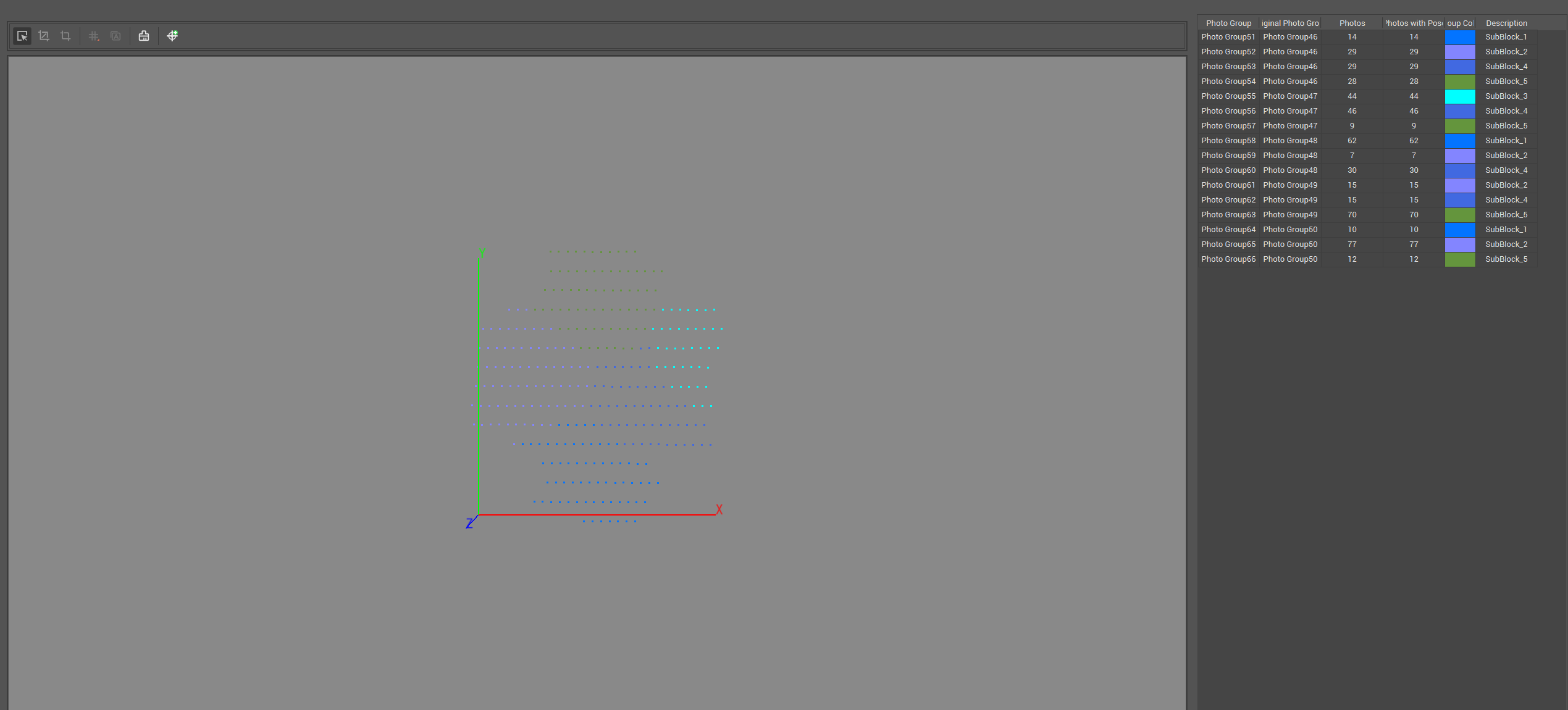
The image below shows the Get3D Mapper Data Manage interface, with different colors indicating different AT blocks.

<figure><img src="/files/O2taavpo4rZVxWG6m4U5" alt=""><figcaption></figcaption></figure>

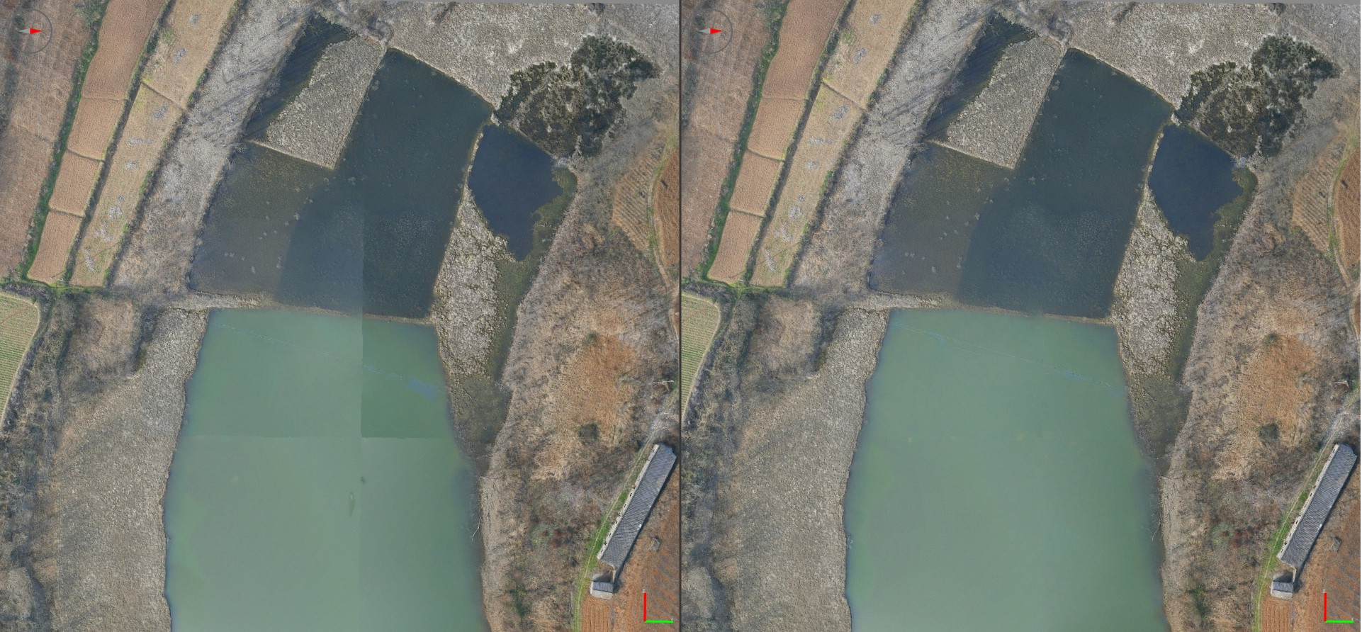
The left image shows before optimization, and the right image shows after optimization.

<figure><img src="/files/LN0L8j2oSn0OJNURj5vn" alt=""><figcaption></figcaption></figure>

<figure><img src="/files/bU0J4jgGI9deDlnkpuF0" alt=""><figcaption></figcaption></figure>

<figure><img src="/files/Kix75J9I6v4pCjMFAeNq" alt=""><figcaption></figcaption></figure>

<figure><img src="/files/OU4RZmlMv4lQ6tL7C0GN" alt=""><figcaption></figcaption></figure>

<figure><img src="/files/cn9Ibuhv1va1P1XHvRfs" alt=""><figcaption></figcaption></figure>

<figure><img src="/files/ZQp752KjMFh1aQODR2Pw" alt=""><figcaption></figcaption></figure>

<figure><img src="/files/VR3Ok6V9vN3eNhZdGfks" alt=""><figcaption></figcaption></figure>

<figure><img src="/files/anl3MIbepqYIK7nt2Wng" alt=""><figcaption></figcaption></figure>

<figure><img src="/files/yNlLRw7VkMNKCzcnYgZC" alt=""><figcaption></figcaption></figure>

<figure><img src="/files/XTqgRlxCHFEpd0eiG5Zl" alt=""><figcaption></figcaption></figure>

<figure><img src="/files/5f9MJvYfFUpcNaDt8s3V" alt=""><figcaption></figcaption></figure>

### 4.4 Optimize by Tie Points

This optimization targets small-scale layering issues that automated AT cannot resolve. By adding tie points in the layered area and marking as many visible photos as possible. If the RMS reprojection error exceeds 3 pixels or the reprojection error(relative) of some photos exceeds 5 pixels, the AT relative accuracy in that area is abnormal, leading to structural layering in the model. This operation helps assess AT relative accuracy.\
The processing flow is as follows:

<figure><img src="/files/v3j5FhbNVX3NN6pFCcv4" alt="" width="369"><figcaption></figcaption></figure>

Select Optimize by Tie Control Points, and the remaining parameters can be submitted with defaults.

<figure><img src="/files/wnk5kfZeivwD9W9s973P" alt=""><figcaption></figcaption></figure>

After adding the tie points, use these points to optimize AT.

The left image shows before optimization, and the right image shows after optimization.

<figure><img src="/files/gaXltw5R9cwIYPVHbp8u" alt=""><figcaption></figcaption></figure>

## 5 Common AT Problems

### 5.1 Camera Intrinsic Parameters

#### 5.1.1 Camera Intrinsic Parameters Inconsistency

The software displays a warning about inconsistent camera intrinsic parameters when the parameters for a photo group do not match the parameters acquired by the software. There are two solutions:

Solution 1: Organize the photos by resolution.

Solution 2: Re-import the photos, selecting the Add Ground Photos.

#### 5.1.2 Focal Length Inconsistency

In Get3D Mapper, all photos in a group should use the same set of camera intrinsics. When importing photos, group them by folder. During data collection, if different devices or focal lengths are used, or if automatic photo rotation occurs, make sure to manually place photos with different parameters in separate folders.

### 5.2 Shadow Changes

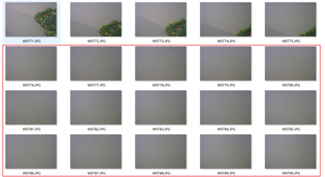
Significant shadow variations caused by lighting changes during aerial photography can lead to large amounts of photo loss in AT, especially when flights are captured in the morning and afternoon. If all photos in one flight are lost at the seam between two flights, you can copy the relative orientation AT results, retain only the vertical images, and check the seam areas between the two flights.

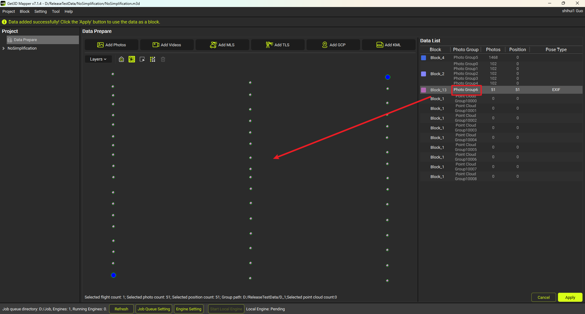
Case: Pink and bright green represent two different flights. In the following images, the tenth flight line from the bottom (highlighted in the red box) has no photos in the net.

<figure><img src="/files/e1vjfABeKrgcXl1Ya26V" alt=""><figcaption></figcaption></figure>

<figure><img src="/files/S0fC6AAMps9ulaTpaS6N" alt=""><figcaption></figcaption></figure>

The following image shows adjacent original photos with significant shadow variation, where the overlapping areas appear completely different on the photos.

<figure><img src="/files/nNFRQMNeaO4XqWYOr9WF" alt=""><figcaption></figcaption></figure>

Solution:

Office Work Solution: Perform separate AT processing for the upper and lower sections, then use control points to merge the two AT blocks.

Field Work Solution: Re-fly and re-collect data to resolve the issue.

Field Work Recommendations:

Photo loss in AT processing is caused by issues during data collection. When collecting data in the field, try to avoid collecting the data of neighboring flights separately in the morning and afternoon of the same day, especially on sunny days with large light difference.


# Software Overview

This section will provide a detailed introduction to the interface and operation of Get3D Mapper.

Get3D Mapper software contains two modules: Get3D Mapper (UI for user to operate) and Get3D Engine runs at background (algorithms for automatic modeling).


# Get3D Engine

Get3D Engine is a work module, running in the background processing tasks, can be online cluster processing jobs.

## 1 Principles of Engine

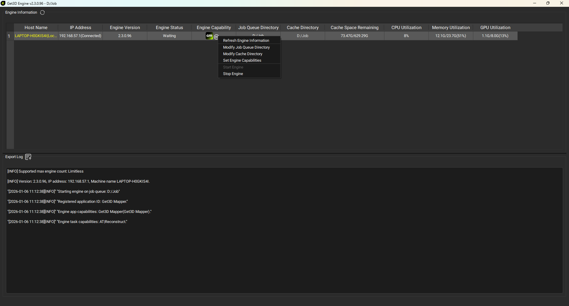
Get3D Engine features a monitoring function for quickly checking engine status, utilization, and modifying settings. Users can adjust configurations such as the "job queue directory," "cache directory," "engine capabilities," and control the engine with "start/stop" options.

* <mark style="color:purple;background-color:purple;">**Job Queue Directory:**</mark> Defines the job path of the current project, the jobs submitted by the current project are stored under this path, waiting for the engine to accept the processing.
* <mark style="color:purple;background-color:purple;">**Cache Directory:**</mark> Stores temporary files during job processing, the path needs to be set to the local disk.

In the Get3D Mapper main interface, the **Job Queue Directory** is used to store submitted jobs. The Get3D Engine retrieves jobs submitted by Get3D Mapper from the **Job Queue Directory**. The engine reads job information (e.g., AT\_job/Reconstruction\_job), processes the jobs, and outputs the results.

<figure><img src="/files/agfIKcoBOFtEvXIhAhaq" alt=""><figcaption><p>Job Queue Setting</p></figcaption></figure>

<figure><img src="/files/QHeHUd09ltevSaqYDdZA" alt=""><figcaption><p>Engine Setting</p></figcaption></figure>

## 2 Engine Monitoring Panel

The Engine Monitoring Panel at the bottom of Get3D Mapper displays the job queue and engine status.

<figure><img src="/files/qt9gm5N2GHYaWjN1qyKE" alt=""><figcaption><p>Engine Monitoring Panel</p></figcaption></figure>

<table><thead><tr><th width="182">Function</th><th>Description</th><th data-hidden></th></tr></thead><tbody><tr><td>Job Queue Directory</td><td>Current job queue directory, where the project's jobs are stored.</td><td></td></tr><tr><td>Engines</td><td>The number of engines in the current job queue directory.</td><td></td></tr><tr><td>Running Engines</td><td>The number of running engines in the current job queue directory.</td><td></td></tr><tr><td>Refresh</td><td>Refresh engine status</td><td></td></tr><tr><td>Job Queue Setting</td><td>Set the job queue for project. Cannot be changed when engine is running.</td><td></td></tr><tr><td>Engine Setting</td><td>Set the job queue for the engine to receive jobs.</td><td></td></tr><tr><td>Start Local Engine</td><td>Start the local engine. </td><td></td></tr><tr><td>Local Engine</td><td><p>The status of the local engine includes four states: </p><p>None: Engine is not started.<br>Pending: Engine is waiting to accept jobs.</p><p>Running: Engine is processing jobs</p><p>Inconsistent path: The engine's job queue directory differs from the project job queue. </p></td><td></td></tr></tbody></table>

## 3 Get3D Engine Interface

Get3D Engine interface has two module: Engine Information and Engine Log

<figure><img src="/files/3tTPo7lqj73pQY4icq6t" alt=""><figcaption><p>Get3D Engine Interface</p></figcaption></figure>

The Engine Information module contains host name, IP address, engine version, engine status, engine capability, job queue directory, cache directory, cache space, CPU utilization, memory utilization, and GPU memory utilization.

<table><thead><tr><th width="260">Function</th><th>Description</th></tr></thead><tbody><tr><td><strong>Host Name</strong></td><td>Device name</td></tr><tr><td><strong>IP Address</strong></td><td>Device IP address</td></tr><tr><td><strong>Engine Version</strong></td><td>Get3D Engine version</td></tr><tr><td><strong>Engine Status</strong></td><td>Stop(closed), Waiting(opened without accepting a task), Running(task running), Abnormal (exited abnormally)</td></tr><tr><td><strong>Engine Capability</strong></td><td>Set the engine capability, the engine only processes jobs with this processing capability. AT: extract points, matching, small block bundle, overall bundle; Reconstruction</td></tr><tr><td><strong>Job Queue Directory</strong></td><td>Set directory for engine to receive jobs</td></tr><tr><td><strong>Cache Directory</strong></td><td>Set engine cache directory</td></tr><tr><td><strong>Cache Space Remaining</strong></td><td>Project cache disk, used space/hard drive space</td></tr><tr><td><strong>CPU Utilization</strong></td><td>CPU usage percentage</td></tr><tr><td><strong>Memory Utilization</strong></td><td>Memory, used memory/node memory</td></tr><tr><td><strong>GPU Utilization</strong></td><td>Video memory, used video memory/node video memory</td></tr></tbody></table>

## 4 Get3D Engine Setting

The engine setting function is in the node information list, right-click to jump out, the setting function is shown in the figure below:

<figure><img src="/files/TSu98ygrO16alkxN2Kdy" alt=""><figcaption><p>Set Engine</p></figcaption></figure>

<table><thead><tr><th width="280">Function</th><th>Description</th></tr></thead><tbody><tr><td><strong>Refresh Engine Information</strong></td><td>Refresh engine CPU, memory, GPU utilization, engine status, cache directory space remaining information</td></tr><tr><td><strong>Modify Job Queue Directory</strong></td><td>Modify the job queue directory of engine</td></tr><tr><td><strong>Modify Cache Directory</strong></td><td>Modify the cache directory of project</td></tr><tr><td><strong>Set Engine Capabilities</strong></td><td>Acquire the capability to receive AT/reconstruction jobs</td></tr><tr><td><strong>Start Engine</strong></td><td>Start accepting jobs</td></tr><tr><td><strong>Stop Engine</strong></td><td>Stop accepting jobs</td></tr></tbody></table>


# Project Tree

This section provides overview of the interface based on the project tree and workflow.

Get3D Mapper is the main user interface, the software project is a tree-like structure, which contains multiple blocks under the project. Different reconstruction frameworks can be created under the blocks according to the requirements. And multiple different types of product results can be submitted under the reconstruction frameworks.

<figure><img src="https://saas.bk-cdn.com/t/8731847e-01c8-438b-9575-3484e4c58acf/u/69b2a8d0-cbbf-402c-adb4-9fad53a9f967/1715390916351/image.png" alt=""><figcaption><p>Project Tree</p></figcaption></figure>

## 1 Data Manage

<figure><img src="/files/D2YWZo1M0ff3me9m01z0" alt=""><figcaption><p>Data Manage</p></figcaption></figure>

<figure><img src="/files/WWRDssWiYvyfZe1Cr8ZO" alt=""><figcaption><p>Data Manage Overview</p></figcaption></figure>

### 1.1 Import Data

1. **Add Images**

Get3D Mapper supports importing aerial photos and ground photos, you can organize your data according to the **file specification**, and choose to import as needed according to the actual scene.

<figure><img src="https://saas.bk-cdn.com/t/8731847e-01c8-438b-9575-3484e4c58acf/u/69b2a8d0-cbbf-402c-adb4-9fad53a9f967/1715647906816/image.png" alt=""><figcaption><p>File Specification</p></figcaption></figure>

After importing the data, the images need to be further positioned to restore their pose. Get3D Mapper supports positioning methods such as EXIF (Exchangeable Image File Format) data and pose files.

<figure><img src="https://saas.bk-cdn.com/t/8731847e-01c8-438b-9575-3484e4c58acf/u/69b2a8d0-cbbf-402c-adb4-9fad53a9f967/1716276632693/%E6%B7%BB%E5%8A%A0%E5%BD%B1%E5%83%8F%E7%95%8C%E9%9D%A2.png" alt=""><figcaption><p>Import Photos and Pose Setting</p></figcaption></figure>

<figure><img src="/files/60hmOIZHGt9dyYrZ1t8c" alt=""><figcaption><p>Import Photos and Pose Setting Inter face Overview</p></figcaption></figure>

**EXIF Positioning**

<mark style="color:yellow;background-color:yellow;">**1) Add photos**</mark>

Select the root directory of the file to import all the photos under the folder.

<figure><img src="/files/mTF8EzmDcLtxib63HzZ4" alt=""><figcaption><p>Import Photos</p></figcaption></figure>

<mark style="color:yellow;background-color:yellow;">**2) Read Exif location**</mark>

Check the Exif information column, select the "exist" photo group, right click to open the menu bar, click **Read Exif** button.

<figure><img src="/files/u0OaR574SbqhYXeU6TxJ" alt=""><figcaption><p>Read Exif</p></figcaption></figure>

<mark style="color:yellow;background-color:yellow;">**3) Query**</mark>

<figure><img src="/files/qMt0q1vEMkOGWuRm0h6x" alt=""><figcaption><p>Quiry</p></figcaption></figure>

<mark style="color:yellow;background-color:yellow;">**4) Progress bar**</mark>&#x20;

<figure><img src="/files/2TEh3Lh44wiZOZ67YS4C" alt=""><figcaption><p>Progress Bar</p></figcaption></figure>

<mark style="color:yellow;background-color:yellow;">**5) Positioning completion**</mark>

After the positioning is completed, "0/2250" is switched to "2250/2250", i.e. each photo in the photo group has positioning information corresponding to it.

<figure><img src="/files/RlvbmnpiRqqMVLaTwIJ6" alt=""><figcaption><p>After Positioning</p></figcaption></figure>

**Pose File Positioning**

<mark style="color:yellow;background-color:yellow;">**1) Add photos**</mark>

<figure><img src="/files/U78NdGnWNWAw2NEw4Say" alt=""><figcaption><p>Import Photos</p></figcaption></figure>

<mark style="color:yellow;background-color:yellow;">**2) Automatic matching of photo groups and pose files**</mark>

* a) Automatic Matching

Pose files are stored in the way shown in the following figure, Pose file name contains keywords such as POS; GPS; RTK; PPK, etc. After importing photos, the photo group will automatically correspond to the pose file.

Tip: Pose file does not contain (POS; GPS; RTK; PPK) keywords, you can set the keywords manually, select the photo group, right-click and use the menu bar, automatically search by keywords.

* b) Manual Correspondence

<figure><img src="/files/x6vH3DHcc3tzH9Tdzqh3" alt=""><figcaption><p>Select Pose File</p></figcaption></figure>

<mark style="color:yellow;background-color:yellow;">**3) Selection of the Pose file**</mark>

Batch select multiple groups of photos by right-clicking to open **Select Pose File** in the menu bar.

<mark style="color:yellow;background-color:yellow;">**4) Define the pose format template**</mark>

Set the spatial reference of the Pose, the separator, and the actual meaning of each column ("photo name, longitude, latitude, elevation" or "photo name, east coordinate, north coordinate, elevation").

<figure><img src="https://saas.bk-cdn.com/t/8731847e-01c8-438b-9575-3484e4c58acf/u/69b2a8d0-cbbf-402c-adb4-9fad53a9f967/1716278832234/%E8%AE%BE%E7%BD%AE%E7%BB%8F%E7%BA%AC%E5%BA%A6%E6%A0%87%E9%A2%98%E5%B9%B6%E5%BA%94%E7%94%A8%E5%88%B0%E7%85%A7%E7%89%87%E7%BB%84.png" alt=""><figcaption><p>Define Template for Pose File</p></figcaption></figure>

<mark style="color:yellow;background-color:yellow;">**5) Apply to photo groups**</mark>

After defining the template, click **Apply to Group** to select the photo group.

<figure><img src="/files/bDeBzr1QvcvxwJ5pGG0Q" alt=""><figcaption></figcaption></figure>

<mark style="color:yellow;background-color:yellow;">**6) Positioning completion**</mark>

After the positioning is completed, "0/2250" is switched to "2250/2250", i.e., each photo in the photo group has positioning information corresponding to it.

<figure><img src="/files/UVAm8I1zMZbK8asywlA5" alt=""><figcaption><p>Apply Successfully</p></figcaption></figure>

2. **Add Video**

Get3D Mapper supports adding videos to get the corresponding video frames and add them to the block image. In the Data Manage interface, click the **Add Video** button, set the input and output file paths, and set the start and end of the extracted video frames as well as the interval time, then you can extract the imported video frames directly.

<figure><img src="/files/kcU2HIgfLc2dXiqxjwgK" alt=""><figcaption><p>Add Video Interface Overview</p></figcaption></figure>

<figure><img src="/files/Nn1ZpPO7NWdHj0Xrz5gn" alt=""><figcaption><p>Select Video File</p></figcaption></figure>

<figure><img src="/files/9nue48t9FwpKOxfyr4xq" alt=""><figcaption><p>Set Video Time</p></figcaption></figure>

<figure><img src="/files/4woNhiftsOtT5GCe0Hsd" alt=""><figcaption><p>Importing</p></figcaption></figure>

<figure><img src="/files/x51wEhTSFcFMBgDZ9Mf2" alt=""><figcaption><p>After Importing</p></figcaption></figure>

3. **Add Mobile Scan**

Get3D Mapper supports the addition of laser point cloud and track line data collected by mobile laser equipment. The software supports laser point cloud modeling alone and laser point cloud fusion modeling with photos.

Support vehicle-mounted, airborne, backpack, and handheld laser point clouds. Laser point cloud supported formats: \*.las, \*.ptx, \*.pts, \*.e57. Trajectory line supported formats: \*.txt, \*csv.

<mark style="color:yellow;background-color:yellow;">**1) Open the Add Mobile Point Cloud interface**</mark>

<figure><img src="/files/12VKU6cbgMaGbUR6JVoK" alt=""><figcaption><p>Add Mobile Scan</p></figcaption></figure>

<figure><img src="/files/8B6bD2OXEB9CYLBM8a3J" alt=""><figcaption><p>Add Mobile Scan Interface</p></figcaption></figure>

<figure><img src="/files/gJ3mEF7pBeJSxlO2zYre" alt=""><figcaption><p>Add Mobile Scan Overview</p></figcaption></figure>

<mark style="color:yellow;background-color:yellow;">**2) Setting up the laser point cloud spatial reference**</mark>

<figure><img src="/files/P0YFJ4IhikhWEZgjWwYt" alt=""><figcaption><p>Select Coordinate System for Point Cloud</p></figcaption></figure>

<mark style="color:yellow;background-color:yellow;">**3) Selection of mobile laser point cloud data**</mark>

<figure><img src="/files/etRI5baxBAiQ3omqJ0O7" alt=""><figcaption><p>Select Point Cloud File</p></figcaption></figure>

<mark style="color:yellow;background-color:yellow;">**4) Importing trajectory lines**</mark>

<figure><img src="/files/8CLfJmjXhfXhcQlLND4b" alt=""><figcaption><p>Select Trajectory File</p></figcaption></figure>

<mark style="color:yellow;background-color:yellow;">**5) Define the trajectory line**</mark>

Set the spatial reference of the track line, the separator, and the actual meaning corresponding to each column ("GPS time, longitude, latitude, elevation" or "GPS time, east coordinate, north coordinate, elevation").

<figure><img src="/files/muCCGKypEvsWfCiSOK4b" alt=""><figcaption><p>Define Trajectory Fields</p></figcaption></figure>

&#x20;<mark style="color:yellow;background-color:yellow;">**6) Enquiry**</mark>

Whether you need to check for data matching.

<figure><img src="/files/P4v7r1zNoBZ7xfzdhHT3" alt=""><figcaption><p>Quiry</p></figcaption></figure>

<mark style="color:yellow;background-color:yellow;">**7) Check the matching results**</mark>

Laser point cloud check contains laser point position and track line position matching; laser point cloud time and track line time matching. And display the matching status.

<figure><img src="/files/1JBbMOndLu9k2r3bAz5v" alt=""><figcaption></figcaption></figure>

<mark style="color:yellow;background-color:yellow;">**8) Data Manage interface display**</mark>

<figure><img src="/files/glntAiEgjaV9s7OcUhhL" alt=""><figcaption><p>After Importing Point Cloud</p></figcaption></figure>

4. **Add Static Scan**

Get3D Mapper supports adding laser point cloud and center data collected by a stationary laser equipment. The software can support laser point cloud modeling alone and laser point cloud and photo fusion modeling. The following formats are supported: \*.las, \*.ptx, \*.pts, and \*.e57. The station center supports manual input or import of \*.txt format files.

<figure><img src="/files/gCfO3YpBB2hVg3Q9tEoS" alt=""><figcaption><p>Add Static Scan</p></figcaption></figure>

<figure><img src="/files/rWv7Jggppostewpt0Mm9" alt=""><figcaption><p>Add Static Scan Interface</p></figcaption></figure>

<figure><img src="/files/AcNACf8MkhG38CHJUf5F" alt=""><figcaption><p>Add Static Scan Overview</p></figcaption></figure>

<mark style="color:yellow;background-color:yellow;">**1) Click Add Static Scan**</mark>

<mark style="color:yellow;background-color:yellow;">**2) Select the point cloud coordinate system**</mark>

<mark style="color:yellow;background-color:yellow;">**3) Add Point Cloud**</mark>

<figure><img src="/files/SnMX8feQszULV18dZv5U" alt=""><figcaption><p>Select Point Cloud File</p></figcaption></figure>

<mark style="color:yellow;background-color:yellow;">**4) Add Station Center:**</mark>

There are two ways to add station center coordinates:

One is to manually add station center coordinates on the right side of the point cloud list.

The other is to click **Add Station Center**, import the center of the station coordinates file. File samples such as the figure below, including the point cloud name, x, y, z arrangement, separated by a space in the middle:

<figure><img src="/files/zp2x9UTdHSv6yIXUsuZC" alt=""><figcaption><p>Station Center File</p></figcaption></figure>

<figure><img src="/files/kQknlyvYp0TTL9N9lyHD" alt=""><figcaption><p>Select Station Center File</p></figcaption></figure>

<figure><img src="/files/OzJaCYrc5i17MMhdlSwn" alt=""><figcaption><p>Station Center Setting</p></figcaption></figure>

If there is no station center coordinates, the software can automatically calculate, uncheck the Define station center.

### 1.2 Import Reference

1. **Add Control Points**

Add control points to the **Data Manage** view, as a block split reference, or as an imported photo data integrity reference.

<mark style="color:yellow;background-color:yellow;">**1) Open Add Control Point**</mark>

<figure><img src="/files/e5Nc584OTXfHRiJM8g5y" alt=""><figcaption><p>Add Control Point</p></figcaption></figure>

<mark style="color:yellow;background-color:yellow;">**2) Selection of control point file**</mark>

<figure><img src="/files/ZV8B4RLteHuDLBerVme8" alt=""><figcaption></figcaption></figure>

<mark style="color:yellow;background-color:yellow;">**3) Define the control point file format**</mark>

Set the spatial reference and delimiter. Define the control point file as "point name, longitude, latitude, elevation" or "point name, east coordinate, north coordinate, elevation".

<figure><img src="/files/5W59TaHtInjUqlpOiV31" alt=""><figcaption><p>Define Control Point Fields</p></figcaption></figure>

The following is an introduction to the interface functions:

<figure><img src="/files/tBacAATIkWuT31O8UHSb" alt=""><figcaption><p>Add Control Point Interface Overview</p></figcaption></figure>

<mark style="color:yellow;background-color:yellow;">**4) Successfully importing control points**</mark>

<figure><img src="/files/W2LSgJDiClzX04ir4PD2" alt=""><figcaption><p>After Importing Contro Points</p></figcaption></figure>

<mark style="color:yellow;background-color:yellow;">**5) Clear control points**</mark>

The added control points can be clear by click **Clear Control Points**.

<figure><img src="/files/EY3yuRJy9HHn9eSqyh7E" alt=""><figcaption><p>Clear Control Points</p></figcaption></figure>

2. **Add KML**

* **KML, which stands for Keyhole Markup Language and was originally developed by Keyhole Corporation, is a coding specification based on XML syntax and formatting for describing and preserving geographic information such as points, lines, images, polygons, and models.**&#x20;

<figure><img src="/files/eVCZYpI39fGT61ZbYrzC" alt=""><figcaption><p>Add KML</p></figcaption></figure>

<mark style="color:yellow;background-color:yellow;">**a. Add the KML file**</mark>

Add a range line to the Data Manage view as a reference to the data integrity of the imported photos.

Range line reference data can be imported after tilt or other multi-source data is imported in the data management interface.

<mark style="color:yellow;background-color:yellow;">**b. Select the background KML file**</mark>

<figure><img src="https://saas.bk-cdn.com/t/8731847e-01c8-438b-9575-3484e4c58acf/u/69b2a8d0-cbbf-402c-adb4-9fad53a9f967/1716279098545/%E8%AE%BE%E7%BD%AE%E6%96%87%E4%BB%B6%E6%89%80%E5%9C%A8%E8%B7%AF%E5%BE%84%E5%B9%B6%E9%80%89%E6%8B%A9.png" alt=""><figcaption></figcaption></figure>

<figure><img src="https://saas.bk-cdn.com/t/8731847e-01c8-438b-9575-3484e4c58acf/u/69b2a8d0-cbbf-402c-adb4-9fad53a9f967/1716279161933/%E6%88%90%E5%8A%9F%E6%B7%BB%E5%8A%A0%E8%8C%83%E5%9B%B4%E7%BA%BF.png" alt=""><figcaption><p>After Adding KML</p></figcaption></figure>

<mark style="color:yellow;background-color:yellow;">**c. Delete KML line**</mark>

The imported range line data can be cleared by clicking **Clear KML**.

<figure><img src="https://saas.bk-cdn.com/t/8731847e-01c8-438b-9575-3484e4c58acf/u/69b2a8d0-cbbf-402c-adb4-9fad53a9f967/1716279122939/%E7%82%B9%E5%87%BB%E6%B8%85%E9%99%A4%E8%8C%83%E5%9B%B4%E7%BA%BF%E6%8C%89%E9%92%AE%E4%B8%80%E9%94%AE%E6%B8%85%E7%A9%BA%E5%AF%BC%E5%85%A5%E7%9A%84%E8%8C%83%E5%9B%B4%E7%BA%BF.png" alt=""><figcaption><p>Delete KML File</p></figcaption></figure>

### 1.3 Edit

After adding photos and pose data, in the Data Manage view each photo is expanded according to the corresponding position (x y z), and editing operations such as selecting, truncating, framing, and deleting can be performed.

<figure><img src="/files/0CABht2oDQRDsBuavpLr" alt=""><figcaption><p>Edit Function Overview</p></figcaption></figure>

### 1.4 View

The photo visualization interface in the Data Manage, in the photo group list view, you can rename, block and other operations on the positioned photo group data.

<figure><img src="/files/E5uT7mGu1ApQ97UXULnE" alt=""><figcaption><p>View Function Overview</p></figcaption></figure>

## 2 Aerial Triangulation

Aerial Triangulation consists of two parts, the Relative Orientation and the Absolute Orientation.

* ***Relative Orientation:*** Relative Orientation, refers to the work of restoring or determining the relative relationship of the image pairs at the time of photography, i.e. solving the work of the relative orientation elements of the stereo image pairs. It is through the observation of the image of the object in different viewpoints of the position of the relationship to determine the internal and external parameters of the camera, the relative orientation of the stereo image pairs is to restore the photography of the two neighbouring image beams of the interrelationship between the two, so that the same name of the light pairs to the intersection of the light pairs.
* ***Absolute Orientation*****:** Absolute Orientation is through the measurement of the ground control points, the image and the ground coordinate system for contact. It uses the known ground control points to translate, rotate and scale the relatively orientated three-dimensional geometrical model to incorporate it into the ground photogrammetric coordinate system, and to improve the absolute accuracy of AT through the control points.

### 2.1 Aerial Triangulation Settings

After the photos are imported into the software, the first step is relative orientation to recover the internal and external parameters of each photo. The second step is absolute orientation to improve the absolute accuracy of the Aerial Triangulation.

**Aerial Triangulation parameters setting:**

<figure><img src="/files/yD3e6fXkaTawkURZuM66" alt=""><figcaption><p>AT Basic Settings Overview</p></figcaption></figure>

The preset options, which contain more settings, are shown below:

<figure><img src="/files/1ue9wV7qxUUjUhQht8va" alt=""><figcaption><p>AT Advanced Settings Overview</p></figcaption></figure>

For a detailed description of the AT Setting, please see the **Aerial Triangulation Setting Instruction** document.

<figure><img src="/files/27BHNPGfMXtk21iNY0eI" alt=""><figcaption><p>AT Setting Tips</p></figcaption></figure>

### 2.2 View Task Details

To check the detailed progress of the AT, including the time for each sub-task and the total time consumed.

<figure><img src="/files/1yQDbRLRebxBbAbvj9xv" alt=""><figcaption></figcaption></figure>

### **2.3 Aerial Triangulation 3D View**

The content displayed in the Aerial Triangulation 3D view includes information such as photo pose, tie points, control points, laser point cloud, and laser trajectory lines.

<figure><img src="/files/hCcc5Lbd6PtGDhP7dyVL" alt=""><figcaption><p>AT 3D View Overview</p></figcaption></figure>

### **2.4 AT Report**

For projects that have completed Aerial Triangulation, an Aerial Triangulation report can be generated by clicking on **View AT Report** in the block view.

<figure><img src="/files/H2pzuaa7IqiRXYx0RHIv" alt=""><figcaption><p>View AT Report</p></figcaption></figure>

For projects with large image data, the process of generating this report takes some time.

The AT report mainly includes the following parts: **project overview, camera calibration, photo information, tie point information,** and **control points**.

<figure><img src="/files/fNk9DblwfjNjB5kzLlxS" alt=""><figcaption><p>AT Report Overview</p></figcaption></figure>

**Project overview:** It contains the project where Aerial Triangulation is located, the running time, the number of photos, the number of control points, the number of photos entering the network, the photo ratio in net, the number of tie points, the average resolution of tie points, and the re-projection error of tie points.

<figure><img src="/files/YrK8bFlRAH9VemWtjoDL" alt=""><figcaption><p>Block Overview</p></figcaption></figure>

**Camera calibration:** A detailed list of information on the internal and external parameters and distortion coefficients of the camera set, which are used to assess the calibration accuracy of the camera.

**Photo information**: Schematic of the offset distance of the camera position from the original POS data, schematic of the re-projection error for each photo, the number of connection points observed by the camera, and the scene coverage. Corresponding connection points, re-projection error for each photo.

<figure><img src="/files/sR0HExlpYGGZ2q4f9l51" alt=""><figcaption><p>Photo Information</p></figcaption></figure>

**Tie point information**: Observation count of tie points, re-projection error of tie points.

<figure><img src="/files/OxHJt9tsNZPBhMgbQ8t7" alt=""><figcaption><p>Tie Points Information</p></figcaption></figure>

**Control points**: coordinates and error information of each control point.

### 2.5 AT Indicators

#### 2.5.1 Rate of Calibrated Photos

Rate of calibrated photos is an important indicator in AT, but not the sole criterion for evaluating AT quality. The results should be assessed based on the actual data. Here are common reasons for photos not calibrated:

① Water Surface Photo Loss

Blue points in the left image show photos that weren’t calibrated. In the right image, the red box highlights the missing photos.

<div><figure><img src="/files/eoMsbaPH3CZ1Vrj2FYXp" alt=""><figcaption></figcaption></figure> <figure><img src="/files/ibMPcdWowlob6HXUlgVC" alt=""><figcaption></figcaption></figure></div>

② Mountainous Area Photo Loss

Blue points in the left image show photos at the edge of the flight area. It is too close to the ground. And the terrain is forest. All these factors may cause some photos not calibrated, which is normal and does not affect modeling within the survey area.

<div><figure><img src="/files/gMNt3jFUrgsPgJulgCk3" alt=""><figcaption></figcaption></figure> <figure><img src="/files/4iU6M8V2zWgFcwBJhJMN" alt=""><figcaption></figcaption></figure></div>

#### 2.5.2 Control Point Accuracy

The absolute orientation in AT uses control point information to adjust camera position and orientation, improving the absolute accuracy of the AT. Check the result of absolute orientation. If the error of X/Y/Z is under 0.01m, the absolute accuracy is high.

#### 2.5.3 Checkpoint Accuracy

Checkpoints assess the accuracy of the AT results. By comparing checkpoint coordinates with AT results, the positional error can be calculated, providing a quantitative evaluation of the AT accuracy. The accuracy requirements of the checkpoints are based on the absolute accuracy requirements of the actual model. For example, if the required planar accuracy is better than 0.1m and the elevation accuracy is better than 0.15m, the error of the checkpoints (X/Y/Z) should meet these requirements.

## 3 Reconstruction

Create a **New 3D Reconstruction** or **New 2D Reconstruction** spatial frame on Aerial Triangulation (set up spatial references, area of interest ranges, tile divisions, reconstruction memory estimates, and more settings) under which one or more products can be submitted.

<figure><img src="https://saas.bk-cdn.com/t/8731847e-01c8-438b-9575-3484e4c58acf/u/69b2a8d0-cbbf-402c-adb4-9fad53a9f967/1716280307501/%E9%87%8D%E5%BB%BA%E5%8F%82%E6%95%B0%E8%AE%BE%E7%BD%AE%E4%B8%BB%E7%95%8C%E9%9D%A2.png" alt=""><figcaption><p>Reconstruction Spatial Framework</p></figcaption></figure>

### 3.1 Reconstruction Setting

The 2D reconstruction setting is same with 3D reconstruction.

**(1) Spatial Reference System**

The spatial reference system is set to the ENU coordinate system (Local East-North-Up system) by default. Users can change it to an existing or custom-defined coordinate system. Using a consistent spatial reference ensures seamless alignment of tile boundaries in subsequent reconstruction processes.

**Note:** The reconstruction coordinate system supports only projected coordinate systems, not geodetic coordinate systems.

**(2) Region of Interest**

There are multiple ways to set the region of interest: quickly setting the range, editing the region in the view, or importing KML boundary lines.

<mark style="color:yellow;background-color:yellow;">**Quickly set the range:**</mark>

**Adjust to Tie Points**: The area of interest ranges to the largest outer enclosing box that contains all tie points.

**Adjust to Camera**: The area of interest ranges to the largest outer enclosing box containing all cameras.

<mark style="color:yellow;background-color:yellow;">**Edit the region in the view:**</mark>

Select **Edit Region**, then drag the faces of the bounding box to define the area.

<figure><img src="/files/aX09c9iTkZD9vfKOcrWf" alt=""><figcaption><p>Edit Region</p></figcaption></figure>

<mark style="color:yellow;background-color:yellow;">**Importing KML boundary lines:**</mark>

Select **Import KML**, and import the the pre-drawn KML boundary line.

<figure><img src="/files/z5q8zvxTfVsDxy7pkvWa" alt=""><figcaption><p>Import KML</p></figcaption></figure>

**(3) Tiling**

<figure><img src="https://saas.bk-cdn.com/t/8731847e-01c8-438b-9575-3484e4c58acf/u/69b2a8d0-cbbf-402c-adb4-9fad53a9f967/1716280336803/%E7%93%A6%E7%89%87%E5%88%92%E5%88%86%E6%A8%A1%E5%BC%8F.png" alt=""><figcaption><p>Tilling Mode</p></figcaption></figure>

* Split Mode: Planar grid division, 3D grid division, no division.
* Tile Size: Set the tile length. There is a proper tile edge length by default (related to AT resolution, related to GSD), user can customize the tile size.
* Tile Overlap: Set the overlap length of neighbouring tiles. When using tile reconstruction, in order to avoid gaps between tiles, set the width of overlap between tiles.
* Origin XYZ: Set the coordinates of the origin of the tiles.
* Preview in Real Time: After modifying the parameters, display the updated result in the 3D view in real time.
* Discard Empty Tiles: Tiles without tie points are not reconstructed.

<figure><img src="https://saas.bk-cdn.com/t/8731847e-01c8-438b-9575-3484e4c58acf/u/69b2a8d0-cbbf-402c-adb4-9fad53a9f967/1715761618750/image.png" alt=""><figcaption><p>Planar Grid Division</p></figcaption></figure>

<figure><img src="https://saas.bk-cdn.com/t/8731847e-01c8-438b-9575-3484e4c58acf/u/69b2a8d0-cbbf-402c-adb4-9fad53a9f967/1715761625265/image.png" alt=""><figcaption><p>3D Grid Division</p></figcaption></figure>

**(4) Save and Load**&#x20;

Save: save the reconstruction space frame settings, including space reference, tile division origin, tile size, tile overlap.

Load: load the reconstruction space frame settings.

**(5) Memory Estimation**&#x20;

Single tile using the maximum memory value prediction, tile reconstruction requires the size of the computer memory related to the tile size (the larger tile, the larger the computer hardware memory required), according to the computer memory to determine the size of the tile division, the prediction of too much memory will lead to the failure of the tile reconstruction.

For example, if you have 64GB of computer memory, you can adjust the tile length, set the tile estimated memory to 30GB, and actually divide the largest tile.

**(6) Copy Setting**&#x20;

Copy other reconstruction parameters under the same project contains space reference, tile division origin, tile size, and so on.

### 3.2 More Settings

<figure><img src="/files/PzdXKzWbQVJiwz45hhNE" alt=""><figcaption><p>More Reconstruction Settings</p></figcaption></figure>

More Reconstruction Settings interface allows you to set the **Point Cloud Generation**, **Mesh Generation**, **Texture Fill** and **2D Reconstruction Hole-Fill Mode** in the reconstruction step. Different preset reconstruction modes can be set in **More Setting** for different modeling scenarios:

l General: The default mode is a balance between model quality and processing efficiency and is suitable for most reconstruction scenarios.

* **General**: The default mode is a balance between model quality and processing efficiency and is suitable for most reconstruction scenarios.
* **High Quality**: High quality mode generates more structural details, consumes more memory and time (about 4 times longer than general mode) to process the same data, and is suitable for fine modelling of small scenes.
* **High Efficiency**: High-efficiency mode pursues high-efficiency modeling quality, the quality of the model will be reduced, the demand for memory and storage resources is small, and the time consumed is short, suitable for large scenes, and the geometric accuracy requirement is not high for rapid modeling scenarios.
* **Define**: Users can choose suitable reconstruction parameters according to their own needs.

<mark style="color:yellow;background-color:yellow;">**① Point Cloud Generation**</mark>

Mainly image dense matching strategy, photo selection strategy, matching strategy, matching accuracy.

<mark style="color:yellow;background-color:yellow;">**② Mesh Generation**</mark>

**Topology Construction:**

* 3D mesh: suitable for most model reconstruction cases.
* 2D mesh: suitable for downward looking image modeling.

**Mesh Simplification:**

* Light: low simplification effort, denser triangular mesh, more (valid and invalid) geometric details, larger data volume.
* Normal: moderate strength of simplification, with a balance of data size and (valid and invalid) geometric details.
* Strong: strong simplification, sparser triangular mesh, largely filtered (valid, invalid) geometric details, smaller data size.

**Mesh Optimization：**

If selected, the 3D model contains more details.

**Seam Optimization：**

Topology optimisation of the geometry between tiles can effectively avoid gaps between tiles.

<mark style="color:yellow;background-color:yellow;">**③ Texture Fill**</mark>

* Automatic Interpolation: Automatically fills texture gaps using surrounding textures.
* AI Repair: Utilizes AI algorithms to intelligently restore missing textures.
* Solid Color: Fills missing areas with a uniform color.

<mark style="color:yellow;background-color:yellow;">**④ 2D Reconstruction Hole-Fill Mode**</mark>

DSM/DOM Fill Hole Mode: Adaptive fill and full fill

### 3.3 Reconstruction 3D View

<figure><img src="/files/MN3SGeVczrONtAtJL1a3" alt=""><figcaption><p>Reconstruction 3D View</p></figcaption></figure>

* Layers show/hide: Show/hide region of interest, tile, camera, tie point, point cloud, control point.
* Home: Reset the 3D view.
* Camera +: increase the size of the camera in the 3D view.
* Camera -: increase the size of the camera in the 3D view.
* Edit Region: Manually adjust the reconstruction range in the 3D view, select and then determine the area of interest, i.e. the modeling area, by extruding and stretching the box.
* Import KML: Import KML range for reconstruction range constraints, output 2D and 3D model results can be output by range line shape.
* Export Tile Boundary KML: For the selected tile, export tile boundary as KML file.

## 4 Product

### 4.1 3D Reconstruction--Product

Get3D Mapper can output 3D model products in OSGB and OBJ formats, 3D point cloud products in LAS, TXT, ASC and E57 formats, DOM products in TIFF and JPG formats, and DSM products in TIFF and ASC formats.

Several different types of products can be submitted under the same reconstruction framework.

<figure><img src="/files/KvCCSOIQIQun4bgvwGln" alt=""><figcaption><p>Product Interface</p></figcaption></figure>

<mark style="color:yellow;background-color:yellow;">**① 3D model product**</mark>

After the Aerial Triangulation processing is completed and the reconstruction settings are finished, you can submit the 3D model products in OSGB and OBJ formats for generation.

Select the output format, texture source, texture quality, maximum texture size, and the way to adjust texture.

<figure><img src="/files/byz64toM4oCwf0pk94n6" alt=""><figcaption><p>3D Model Settings</p></figcaption></figure>

* **OBJ**: OBJ is a 3D model file format for model editing and browsing. The .obj file mainly contains information about the vertices, normals, texture coordinates, and faces (triangles or polygons formed by vertices) of the 3D model. The \*.mtl file defines the properties of the materials used in the model, such as colour, gloss, texture mapping, etc. The \*.jpg file is the texture coordinates of the material. \*.jpg files are texture maps.
* **OSGB**: OSGB is a binary format for 3D model data, suitable for applications such as model browsing and real-time rendering.One of the features of the OSGB format is that it can support model representation with multiple Levels of Detail (LOD, Levels of Detail), which allows the system to dynamically load and display model levels of corresponding fineness according to the distance of the observer.

<figure><img src="https://saas.bk-cdn.com/t/8731847e-01c8-438b-9575-3484e4c58acf/u/69b2a8d0-cbbf-402c-adb4-9fad53a9f967/1715844582432/image.png" alt=""><figcaption><p>Structure of Model Formats</p></figcaption></figure>

**Use Multiple Origins:**

When submitting a product, import a multi-origin planning file. It will automatically export the different tiles by origin.

**Select Tiles:**

Select the tiles of interest to be generated into a 3D model or point cloud.

<figure><img src="/files/L7ZGDYY5msgo2Q8UnyXF" alt=""><figcaption><p>Select Tiles</p></figcaption></figure>

<figure><img src="/files/2BAmYN4oWNUlfQLSjycN" alt=""><figcaption><p>Tile Selection Overview</p></figcaption></figure>

<mark style="color:yellow;background-color:yellow;">**② 3D point cloud product**</mark>

After generating a 3D model, the model is sampled to produce a 3D point cloud product.

The software interface allows you to set the point cloud product output format, point cloud source, and resolution.

<figure><img src="/files/NpXHdAUxOyA0MYls2EYG" alt=""><figcaption><p>Point Cloud Settings</p></figcaption></figure>

<mark style="color:yellow;background-color:yellow;">**③ 2D product**</mark>

After generating the 3D model, the model is sampled to generate DOM and DSM products.

The software interface allows you to set the sampling distance, image dimension, DOM product format, and DSM product format.

<figure><img src="/files/HQ5hfjFyqRGSyJTjVATm" alt=""><figcaption><p>2D Product Settings</p></figcaption></figure>

**Select Grids:**

Select the grids, which correspond to the grid divisions set up for the 3D reconstruction spatial frame.

Selection method is same with selecting tiles. The view shows areas that have not been reconstructed, have been reconstructed, and have been selected.

<figure><img src="/files/calcw9p0jrO6MzP4CJW1" alt=""><figcaption><p>Select Grids</p></figcaption></figure>

### 4.2 2D Reconstruction--Product

The software interface allows you to set the resolution, compression type, DOM product format, and DSM product format.

<figure><img src="/files/JUr3GfD3cqMM7KfSvSSN" alt=""><figcaption><p>2D Product Interface</p></figcaption></figure>

<figure><img src="/files/GpdofrQZifhWZQ6AL91K" alt=""><figcaption><p>Products of 2D Reconstruction</p></figcaption></figure>

**Select Grids:**

Select the grids, which correspond to the grid divisions set up for the 2D reconstruction spatial frame.

Selection method is same with selecting tiles. The view shows areas that have not been reconstructed, have been reconstructed, and have been selected.

<figure><img src="/files/calcw9p0jrO6MzP4CJW1" alt=""><figcaption><p>Select Grids</p></figcaption></figure>

### 4.3 Product Report

In the product interface, you can click **View Product Report**.

<figure><img src="/files/EL3t03gagUyAWdxI9FP7" alt=""><figcaption><p>View Reconstruction Report</p></figcaption></figure>

The product report contains **Project Overview Information** and **Tile Information**.

<figure><img src="/files/YaBQ2yeR9EvPOs8dWLcS" alt=""><figcaption><p>Product Report Overview</p></figcaption></figure>

The product overview contains information about the coordinate system and origin of the modeled tiles, the size of the modeling area, and the time spent on the modeling.

<figure><img src="/files/suTWsp4xmlAi2qatO3pB" alt=""><figcaption><p>Product Overview</p></figcaption></figure>

The tile information includes the runtime and status of each tile.

<figure><img src="/files/K5tpaS3ZYqQjGsNzwAVx" alt=""><figcaption><p>Tile Information</p></figcaption></figure>


# Menu Bar

This section will introduce you to how the functions of the menu are used.

## 1  Project

### 1.1 New Project

After opening Get3D Mapper software, click **New Project** or **Project >New Project** or use the shortcut key "**Ctrl + N**". Open the New Project page. On the New Project page, you can set the project name and project directory. If cluster computing is required, set the project path to the network path.

<figure><img src="/files/YcNsXIxeaedKUbcWdfwG" alt=""><figcaption><p>New Project</p></figcaption></figure>

<figure><img src="/files/1tzRi9lWo9Lp1WyspF6J" alt=""><figcaption><p>New Project page</p></figcaption></figure>

### 1.2 Open Project

Click **Project > Open Project**, select the \*.m3d project file, and click **Open**. You can also open the project by clicking "Project Name.m3d" in the **Recent Projects** list.

<figure><img src="/files/VddFcp1kkjExkwqoeCCm" alt=""><figcaption><p>Open Recent Projects</p></figcaption></figure>

### 1.3 Save Project

Click **Project > Save Project** button or use the shortcut key "Ctrl+S" to save the project information.

### 1.4 Clean Project

Project processing is complete, click the Project > Clean Project function to clean up the completed project. If the project has a task running, you can not perform this operation. It does not contain the product results generated by the software.

<figure><img src="/files/6WqCIomiYWJwJfE5YcV5" alt=""><figcaption><p>Clean Project</p></figcaption></figure>

**① Clean Project Cache**

Project cache includes AT feature point files(KeyPoints folder) and thumbnail file(Preview folder).

**② Clean Block Cache**

Block cache includes AT match files, bundle files and other setting files(Block/Cache folder).

**③ Clean Reconstruction Cache**

Reconstruction cache includes dense matching point files(Block/Reconstruction/cache\_points folder).

**④ Reconstruction Tile Cache**

Reconstruction tile cache includes tile’s midout results(Block/Reconstruction/Tile folder)

**⑤ Clean Reconstruction Log**

Reconstruction log includes production log files(Block/Reconstruction/Productions/Production/Tile folder).

Quickly clean up files by selecting the corresponding cache.

### 1.5 Close Project

Click **Project > Close Project**, and select **Yes** in the pop-up box to close the project.

### 1.6 Exit

Click **Project > Exit** or use the shortcut key "Ctrl+W" to close Get3D Mapper.

## 2 Block

<figure><img src="/files/kdHhMforaHjzGawaANOu" alt=""><figcaption><p>Block Menu</p></figcaption></figure>

### 2.1 Save Block

Perform a save operation for the edited Aerial Triangulation (AT). For example, save the AT results after deleting photos, tie points, or control points.

### 2.2 Import Block

Aerial Triangulation results can be exported to do Aerial Triangulation results backup or re-imported into other projects to use. Get3D Mapper supports the import of Aerial Triangulation formats: \*.xml, \*.xbin.

<figure><img src="/files/XqFduJ34okbHJevHdyEG" alt=""><figcaption><p>Select Block File</p></figcaption></figure>

### 2.3 Export Block

Get3D Mapper supports the export of internally generated data such as tie points, marking points information, etc. in the format of \*.xml, \*.xbin, \*patb. Select the export data type and cilck OK to export.

<figure><img src="/files/i2msHk8IfENTyxJsnLN6" alt=""><figcaption><p>Export Block</p></figcaption></figure>

<figure><img src="/files/ZbNCfwldOy1t71yE0TXw" alt=""><figcaption><p>Export Block Overview</p></figcaption></figure>

<mark style="color:purple;">This feature is usually used to export AT file as</mark> <mark style="color:purple;"></mark><mark style="color:purple;">**.xml**</mark> <mark style="color:purple;"></mark><mark style="color:purple;">file.</mark>

### 2.4 Export Block Map

Export the POS point locations for the specified block in JPG or PDF format.

<figure><img src="/files/najHq4RHSHcKZIy2IS1v" alt=""><figcaption><p>Export Block Map</p></figcaption></figure>

### 2.5 Modify Photo Directory

If the original photo paths have changed, to ensure that the Aerial Triangulation and Reconstruction tasks read these photos properly, you need to update the paths of the photos in the block.

Click **Block > Modify Photo Directory**

<figure><img src="/files/DYE3k6dW2P3o6rrKZscp" alt=""><figcaption><p>Modify Photo Group Directory</p></figcaption></figure>

Click **Refresh** at the bottom of the screen to check before making changes.

* Red: The path of the photos recorded in the block is abnormal, and there is no corresponding photo under the path.
* Green: The corresponding photos can be found in all the photo paths recorded in the block.

<figure><img src="/files/RKuButDr0waQGRLebFbu" alt=""><figcaption><p>Check Image File</p></figcaption></figure>

Double click to select the new path. The photo storage structure has not changed, and other paths can be replaced automatically.

<figure><img src="/files/gjeMhMWnX7DoEPG55eXk" alt=""><figcaption><p>Select New Path</p></figcaption></figure>

For damaged or missing images, you can delete them by clicking **Delete Lost Photos.**

## **3 Setting**

<figure><img src="/files/tCegjKdURFd9cbDpV95O" alt=""><figcaption><p>Setting Menu</p></figcaption></figure>

The settings are related to Get3D Engine. For more details on its introduction and operation, refer to the previous section [**Get3D Engine**](/user-help-center/get3d-mapper/software-overview/get3d-engine).

## 4 Tool

The tool contains two functions: **Merge DOM/DSM**, and **Model Origin Setting**

### 4.1 Merge DOM/DSM

Merge the generated DOM/DSM split images into a whole image. The specific use operation is as follows.

<figure><img src="/files/QkzLD7UIKb1lQaN17ddh" alt=""><figcaption><p>Merge DOM/DSM</p></figcaption></figure>

① Select the corresponding "Block", "Reconstruction" and "Product".

② Select the **DOM** and **DSM** of the products to be merged and set the output path.

③ Input the sample interval.

④ Set the correct coordinate system.

⑤ Click **Merge** button to start merging DOM/DSM.

### **4.2 Model Origin Setting**

For 3D models in OSGB format, due to limitations on decimal precision, data with ground resolutions at the centimeter level may experience a loss of precision when the model's position in the X or Y direction exceeds 10,000 meters from the origin during reconstruction. This can lead to visual issues such as flickering surfaces in the displayed model.

To address this, a model origin should be defined for every 10,000-meter grid to reduce the magnitude of model coordinate values.

&#x20;① Import boundary KML/SHP.

<figure><img src="/files/VExBkcQL2cyDGvKvZkHv" alt=""><figcaption><p>Import KML</p></figcaption></figure>

② Set the initial origin coordinates, gird length and model origin position.

<figure><img src="/files/gRVjPqyezAllExLoOGPQ" alt=""><figcaption><p>Set Intitial Origin</p></figcaption></figure>

③ Model origin view.

<figure><img src="/files/LKtPxvdB6GUJA5gMJRc5" alt=""><figcaption><p>Model Origin View</p></figcaption></figure>

④ Export model origin.

<figure><img src="/files/bMAHcs2n0zpKyPctoo20" alt=""><figcaption><p>Export Model Origin</p></figcaption></figure>

⑤ Import multi-origin file in product setting interface. Tiles will be exported automatically based on the defined origins.

<figure><img src="/files/XcmswZbPJCVcPtEiO21x" alt=""><figcaption><p>Import Multi-Origin File for Product</p></figcaption></figure>

## 5 Help

<figure><img src="/files/c6zp5DRP1f9CQjVXbVfY" alt=""><figcaption><p>Help Menu</p></figcaption></figure>

#### User Maunal

Refer to this manual for guidance on using the software.

#### Update Operation Guide

Software update log and new features introduction file.

**Log Directory**

Software running log

**Dump Direcory**

he software crash dump storage directory. If the software crashes during normal use, send the dump file from this directory to technical support at <mark style="color:purple;">**<support@get3d.ai>**</mark> for assistance.

**About**

Records the software version number, release date, and official Get3D channels.


# Cluster Mode

Get3D Mapper supports multiple computer cluster computing to process project with large number of images.


# Cluster Computing

Here we introduce you how to perform cluster performing and batch management of engine nodes.

<mark style="color:yellow;background-color:yellow;">**Note：**</mark>

<mark style="color:yellow;background-color:yellow;">(1) Before performing cluster computing on multiple computers, please make sure that each computer is connected to same LAN and can connect each other. Each machine has read and write permission to other computers.</mark>

<mark style="color:yellow;background-color:yellow;">(2) Get3D Mapper software contains two modules:</mark> <mark style="color:yellow;background-color:yellow;"></mark><mark style="color:yellow;background-color:yellow;">**Get3D Mapper**</mark> <mark style="color:yellow;background-color:yellow;"></mark><mark style="color:yellow;background-color:yellow;">(UI for user to operate) and</mark> <mark style="color:yellow;background-color:yellow;"></mark><mark style="color:yellow;background-color:yellow;">**Get3D Engine**</mark> <mark style="color:yellow;background-color:yellow;"></mark><mark style="color:yellow;background-color:yellow;">runs at background (algorithms for automatic modeling).</mark>

## 1 Download & Installation

First, download and install Get3D Mapper on each computer.

The Get3D Mapper installation process will automatically accompany the installation of Get3D Engine.

## 2 Login Account & Activate License

After finishing the installation,

(1) Open the Get3D Mapper software on each of the computers,

(2) Log in to your account and activate the licence to each computer.

For more details on license activation, refer to the section [Newbie Guide > License Acquisition](broken://pages/yDVFuzUqyaKailkqs1lw#id-2-license-acquisition)

## 3 Start Engine

Start the engine on all computers:

Click **Setting>Engine Setting** in the menu bar.

Then click **Start Local Engine** to access the Get3D Engine interface.

<figure><img src="/files/VvtSlcUQmqS4UjZesmW5" alt=""><figcaption><p>Engine Setting</p></figcaption></figure>

<figure><img src="/files/VuYBzyKC4iN5z9n5rKXR" alt=""><figcaption><p>Start Local Engine</p></figcaption></figure>

## 4 Create Project

After obtaining license and starting the engine on all computers.

Select a computer as the master computer and create project.

Please set the project path to a **network path** that can be accessed by other computers. Subsequent operations can be completed on the project of this master computer.

<mark style="background-color:yellow;">**Note:**</mark>

<mark style="background-color:yellow;">All operations except</mark> <mark style="background-color:yellow;"></mark><mark style="background-color:yellow;">**Collaborative Marking Ground Control Points**</mark> <mark style="background-color:yellow;"></mark><mark style="background-color:yellow;">can be performed only on the main project of the master computer:</mark>

* <mark style="background-color:yellow;">Creation of the project；</mark>
* <mark style="background-color:yellow;">Import of the images；</mark>
* <mark style="background-color:yellow;">Positioning of the images；</mark>
* <mark style="background-color:yellow;">Submission of the Relative Orientation；</mark>
* <mark style="background-color:yellow;">Submission of the Absolute Orientation；</mark>
* <mark style="background-color:yellow;">Submission of Reconstruction (generation of the 3D mesh model).</mark>

<mark style="background-color:yellow;">Similarly, mobilizing the computational power of each engine node, managing the start or pause of the engine nodes, etc., can be done from a single engine interface.</mark>

For more details on create project, refer to the section [Newbie Guide > Create Project & Open Project](broken://pages/yDVFuzUqyaKailkqs1lw#id-3-create-project-and-open-project)

## 5 Set Job Queue Directory

After creating the project, set the job queue directory for project. Make sure the **Job Queue Directory** to be network path.

<mark style="background-color:yellow;">Note：</mark>

<mark style="background-color:yellow;">There are four paths in the cluster calculation that need to be network paths:</mark>

<mark style="background-color:yellow;">① 【Create & Open Project】  Project Path</mark>

<mark style="background-color:yellow;">② 【Job Queue Setting】 Job Queue Path (for both project and engine)</mark>

<mark style="background-color:yellow;">③ 【Import & Read Image】  Image Path</mark>

For more details on setting job queue, refer to the section [Newbie Guide > Job Queue & Engine Setting](broken://pages/yDVFuzUqyaKailkqs1lw#id-6-job-queue-and-engine-setting)

## 6 Import Image & Positioning

For more details on importing images and positioning, refer to the section [Newbie Guide > Impot Image](broken://pages/yDVFuzUqyaKailkqs1lw#id-4-import-image), [Newbie Guide > Photo Positioning](broken://pages/yDVFuzUqyaKailkqs1lw#id-5-photo-positioning)

## 7 Submit Job & Distribute Engine Nodes

**Job submission:**&#x20;

After completing the image import and positioning, and correctly filling in the Camera Information (Sensor Size and Focal Length), click **Submit AT**.

**Distribute Engine Nodes:**

(1) **Open the engine interface**. In the Engine Information list, you can see the current state of the Engine (**Waiting, Running, Stop**).

<figure><img src="/files/ZMQrjUozzCSNRvYb4yO7" alt=""><figcaption><p>Get3D Engine Interface</p></figcaption></figure>

(2) Select all engines, right click and select **Modify Job Queue Directory**. Set all the engines to the job queue path where the main project submits the job.

<figure><img src="/files/A0wQTM4tz0ZuCxXZD7LE" alt=""><figcaption><p>Modify Job Queue Directory</p></figcaption></figure>

<figure><img src="/files/WrVS67TSv8hwJlpk6sxy" alt=""><figcaption><p>After Modification</p></figcaption></figure>

Once the job queue is set correctly, all engines will start running. You can view the number and status of the running engines either in the engine interface or in the [engine monitoring panel](/user-help-center/get3d-mapper/software-overview/get3d-engine#id-2-engine-monitoring-panel) of Get3D Mapper.


# Collaborative Marking GCPs

This chapter introduces you how to mark GCPs on multiple computers simultaneously.

For a large number of control points in a project, Get3D Mapper supports multiple computers to mark GCPs together to enhance work efficiency.

<figure><img src="/files/YIeA6wOc7abJfqbVU41q" alt=""><figcaption><p>Collaborative Marking GCPs</p></figcaption></figure>

Get3D Mapper supports opening sub-projects on multiple computers, and the only operation that sub-projects can do is to edit control points.

When the main project enters the interface of editing control points, it locks all control points by default.

When the main project releases a portion of the control points, the secondary project can lock that portion of the released control points and perform Mark GCPs operations. When multiple computers have finished collaborating on the marking, click on each computer to save the control point information.

Finally, the main project will update the control point information.

<figure><img src="/files/puNgNVymQEbVFxPdB25W" alt=""><figcaption><p>Operation Pricinple</p></figcaption></figure>

The specific operation is as follows:

1\) In the main project in the submit AT interface click **Edit GCP** to enter the Edit Control Points interface. **Import the control point file** and **select the correct coordinate system**.

2\) Select some control points and click **Unlock**.

<figure><img src="/files/cirzRRM5Dy9CWLriuB2R" alt=""><figcaption><p>Unlock Points</p></figcaption></figure>

<figure><img src="/files/cn21GHWmk0aDbsn8IupQ" alt=""><figcaption><p>After Unlocking</p></figcaption></figure>

3\) Open the project on another computer. When you open it, the default prompt is that the project opened here is a sub-project, and you can only edit control point operations.

<figure><img src="/files/cTKOvWOZ9GxbfvCKbtyp" alt=""><figcaption><p>Prompt</p></figcaption></figure>

<figure><img src="/files/1fxbNnr7G9JfOVFbxb0N" alt=""><figcaption><p>Edit GCP</p></figcaption></figure>

4\) Enter the Edit Control Points screen, click **Update** to see the unlocked control points, and then you can Mark GCPs on the machine after locking it.

<figure><img src="/files/M6aUf2ZV2LffPjYNLyGk" alt=""><figcaption><p>Update</p></figcaption></figure>

<figure><img src="/files/8ddnYhWKkkHvO6fDzW2D" alt=""><figcaption><p>Unlocked Points</p></figcaption></figure>

For more details on marking GCPs, refer to the section [Edit Control Points](/user-help-center/get3d-mapper/getting-started/edit-control-points)

5\) When sub-project has done marking, click **Update** and **Save**.

<figure><img src="/files/8ShgmTRZJf9P6db7MbA7" alt=""><figcaption><p>Update and Save Sub-Project Marking Results</p></figcaption></figure>

6\) After completing all marking points operation, click **Update**, **Save** in the main project to exit this screen.

<figure><img src="/files/hjNGLxAGvc74AJotH6wV" alt=""><figcaption><p>Update and Save All Marking Results</p></figcaption></figure>


# Automatic Block Division

This section will introduce you how to divide block automatically.

For a one-time import of hundreds of thousands of images for aerial triangulation calculation, Get3D Mapper supports automatic division of blocks through algorithms, and the whole process is convenient and efficient without manual effort.

In Aerial Triangulation Setting Interface, select **Auto Split** and set the **block image number**.

<figure><img src="/files/teoy2w8iwH6em26DYmd8" alt=""><figcaption><p>Split Setting</p></figcaption></figure>

The software will quickly and automatically divide the sub-blocks by algorithm.

Dividing sub-blocks helps to improve computing efficiency, increase cluster utilization, and facilitate parallel computing in the cluster.

**Version Before 6.2**

The automatic block division in version 6.2 operates as follows:

For an imported block, select it, right-click it, and click **Split Sub Block**. the Split Photo Group window will pop up.

<figure><img src="/files/wW6sd9RvNPTlH197xe5H" alt=""><figcaption></figcaption></figure>

Select the block, click **Auto Split**, and enter the number of photos you want to include in a single sub-block. Click **Start Split** in the upper right corner.

<figure><img src="/files/sIypDiEsyTSCEBsIJa3w" alt=""><figcaption><p>Split Photo Groups Interface</p></figcaption></figure>

<figure><img src="/files/GW2FaKsA1WnAaCLEpHVj" alt=""><figcaption><p>Auto Split Interface</p></figcaption></figure>

The software will quickly and automatically divide the sub-blocks by algorithm.

<figure><img src="/files/uGtYcrT15NiOD9ojdzSK" alt=""><figcaption></figcaption></figure>

Click **OK** in the lower right corner to finish splitting the sub-blocks.

When a single block contains many images, clicking Submit AT brings up a pop-up that suggests dividing sub-blocks.


# Release Note


# v7.1.5

* Added 3D Gaussian Splatting Modeling.
* Added option to auto-merge DOM/DSM on export.
* Added one-click viewing of 2D production in Get3D Viewer.
* Optimized task runtime display.
* Optimized partial UI and icons.
* Fixed known issues.

## 1 Added 3D Gaussian Splatting Modeling

(1) For blocks that have completed Aerial Triangulation calculations, right-click block and select New 3D Reconstruction or click the New 3D Reconstruction in the right bottom side to enter the Reconstruction screen.

<figure><img src="/files/eYzAB6ImfcW0zFcp0T7Y" alt=""><figcaption><p>New 3DGS Reconstruction</p></figcaption></figure>

(2) Effect

<figure><img src="/files/0iRc5O0xoHYSfCXZVuZQ" alt=""><figcaption><p>Mesh (Left) &#x26; 3DGS (Right)</p></figcaption></figure>

<figure><img src="/files/nKAzM8Pa4ziJAMhX6djy" alt=""><figcaption><p>Mesh (Left) &#x26; 3DGS (Right)</p></figcaption></figure>

## 2 Added option to auto-merge DOM/DSM on export

(1) Two new checkboxes have been added to the 2D output settings. Users can enable or disable the export of merged 2D products.

<figure><img src="/files/J9Eh7I1TE9AW53Xwm49k" alt=""><figcaption><p>Merge DOM/DSM</p></figcaption></figure>

(2) If the Merge DOM and Merge DSM options are selected, an additional MergeDomDsm folder will be generated in the output, containing the merged DOM and DSM results.

<figure><img src="/files/215mLlhFbFSXJxuNiP6J" alt=""><figcaption><p>MergeDomDsm</p></figcaption></figure>

## 3 Added one-click viewing of 2D production in Get3D Viewer

(1) Usage Conditions.

&#x20;     A. Get3D Viewer version V4.1.0 or later must be installed;\
&#x20;     B. Both DOM and DSM outputs must be generated.

(2) Function Description.

When the above conditions are met and tile reconstruction is successful, users can click the Open With Get3D Viewer button to view the 2D products with one click.

<figure><img src="/files/sqcz5IrrY4ANHaW2XEcr" alt=""><figcaption><p>Open with Get3D Viewer</p></figcaption></figure>

## 4 Optimized task runtime display

The task runtime is now displayed in real time and refreshed every minute.

*<mark style="background-color:purple;">Note: The engine must be updated to V4.0.0.</mark>*

<figure><img src="/files/uHzZMLzkyyjHRmw1rblR" alt=""><figcaption><p>Runtime</p></figcaption></figure>

## 5 Optimized partial UI and icons

(1) Edit GCP interface improvements

&#x20;     A.  Added tutorial entry (Help → Tutorial).

<figure><img src="/files/fJuw51xaJf7YiYnuwMjT" alt=""><figcaption><p>Entry of tutorial</p></figcaption></figure>

&#x20;     B. Optimized the photo loading speed settings. When photo file sizes are large and loading is slow, users can set the loading speed to Slow to avoid UI lag.

<figure><img src="/files/ta4s8k2LBKxNHAJPB4O9" alt=""><figcaption><p>Photo loading speed setting</p></figcaption></figure>

(2) Optimization of the 3D reconstruction setting and submit production interface.

<figure><img src="/files/8rG6zSCiWKYKKuduvcuo" alt=""><figcaption><p>3D reconstruction setting</p></figcaption></figure>

## 6 Fixed known issues

(1) Fixed an issue where the linkage with point record was lost during the marking GCP process;

(2) Fixed an issue where the Edit GCP button was locked out incorrectly;

(3) Fixed an issue with the layer visibility toggle in the Spatial Framework view


# v7.1.4

* Fixed the water color adjustment issue.
* Optimized the design of partial interfaces.

## 1 Fixed the water surface color homogenization issue

<figure><img src="/files/YDgh8VZ1nWx8dP1noI4k" alt=""><figcaption><p>Before Optimization (Left) &#x26; After Optimization (Right)</p></figcaption></figure>

## 2 Optimized the design of partial interfaces

(1) Added a new function in the Data List table: double-click the specified Group area (the red box in the figure) to trigger the Zoom to function.

<figure><img src="/files/oTQPIhIWQqa56H71zovH" alt=""><figcaption><p>Zoom to</p></figcaption></figure>

(2) Optimized the design and operation logic of the data import interface.


# v7.1.3

* Added rapid rough registration function for aerial triangulation of images without location metadata and laser point cloud.
* Optimized aerial triangulation algorithm to improve stability and accuracy for images with high geolocation accuracy captured by DJI lenses.
* Optimized laser point cloud modeling process and adjusted reconstruction parameters.
* Optimized software interfaces and icons.

## 1 Added Rapid Rough Registration Function For Aerial Triangulation Of Images Without Location Metadata And Laser Point Cloud

There are deviations in position and scale between the aerial triangulation of images without position metadata and the laser point cloud. You can use the newly added Coarse Registration function in the GCP marking interface to address this and align the aerial triangulation tie points to the laser point cloud.

(1) Result Comparison

&#x20;    a. Before Alignment

<figure><img src="/files/b5PUfjNbHj6IXVhpjPvi" alt=""><figcaption></figcaption></figure>

&#x20;    b. After Alignment

<figure><img src="/files/2PNv9NyqgHDNGeKAPmjK" alt=""><figcaption></figcaption></figure>

(2) Operation Instructions

For aerial triangulation blocks of images without position metadata that contain laser point cloud data:

&#x20;    a. Click the Edit GCP button to access the GCP marking interface;

<figure><img src="/files/Yp0gVmLrVtHgErB3nd8o" alt=""><figcaption></figcaption></figure>

&#x20;    b. Click 3D View → Registration;

<figure><img src="/files/BXESe6i0bPAZo7a70ahz" alt=""><figcaption></figcaption></figure>

&#x20;    c. Access the Coarse Registration interface;

<figure><img src="/files/xwrAbHAoZScHnU7wUWqB" alt=""><figcaption></figcaption></figure>

&#x20;    d. The left side is the laser point cloud view, and the right side is the aerotriangulation tie point view;

&#x20;    e. First pick a point in the left view, then pick a homologous point in the right view. Select at least three pairs of homologous points;

<figure><img src="/files/2vqUUTeU6iqrvhuqR4ck" alt=""><figcaption></figcaption></figure>

&#x20;    f. Click the Preview button to view the alignment result;

<figure><img src="/files/yabvI4vt6FNMKL3aKtRY" alt=""><figcaption></figcaption></figure>

&#x20;    g. Click the OK button to apply the alignment result.

## 2 Optimized the aerial triangulation algorithm to improve the stability and accuracy of aerial triangulation for high-precision position images captured by DJI lenses

(1) Model Comparison (Left: Aerial Image Modeling; Right: Aerial + Low-Altitude Supplementary Image Fusion Modeling)

<figure><img src="/files/zBPZSjm4Z5HXJE3t8U7M" alt=""><figcaption></figcaption></figure>

<figure><img src="/files/lF8IW1qifXU00DmYohQA" alt=""><figcaption></figcaption></figure>

<figure><img src="/files/yCW2CZrqs0L7SylmRn1d" alt=""><figcaption></figcaption></figure>

<figure><img src="/files/UoRvuM3NURVBO2VTyQyn" alt=""><figcaption></figcaption></figure>

<figure><img src="/files/woERIcFjsexBYQF030nF" alt=""><figcaption></figcaption></figure>

(2) Operation Instructions

When more than 50% of the photos in the Block are identified as having high-precision position information, the High Geolocation Accuracy mode will be displayed and checked by default when submitting the aerial triangulation task. This mode significantly improves aerial triangulation stability and accuracy.

<figure><img src="/files/kkdO7szpxUp4TShJbfol" alt=""><figcaption></figcaption></figure>

(3) Method to Determine Whether Photos Have High-Precision Position Information (Only fixed solution positioning with an RTKFlag of 50 provides centimeter-level high-precision position information.)

<p align="center">Table 1 RTK Accuracy Levels</p>

<figure><img src="/files/kzL8BsIqmTQFdtJZYmpJ" alt="" width="375"><figcaption></figcaption></figure>

&#x20;    a. Method 1: MRK file – the last line displays the RTK position accuracy level.

<figure><img src="/files/L3SnvdhN0MuV4dSgRhoe" alt=""><figcaption></figcaption></figure>

<figure><img src="/files/Nr2rNsIev3yuXSCe9TMz" alt=""><figcaption></figcaption></figure>

&#x20;    b. Method 2: Open the photo in text mode (garbled characters are normal), then press Ctrl + F to search for the "RTKFlag" field.

<figure><img src="/files/sZQ3ot12wESEXButlfxg" alt=""><figcaption></figcaption></figure>

(4) Aerial triangulation Results

&#x20;    a. Aerial images and close-range images are processed separately; select them and then merge the blocks.

<figure><img src="/files/hIDb9brzF88WRAmRdjRi" alt=""><figcaption><p>Close-Range Image Aerial Triangulation</p></figcaption></figure>

<figure><img src="/files/J7sUfZwigESIjOlaCTZ6" alt=""><figcaption><p>Aerial Image Aerial Triangulation</p></figcaption></figure>

<figure><img src="/files/ahciA7vXjCyFNEVOqIx0" alt=""><figcaption><p>Merge Block</p></figcaption></figure>

<figure><img src="/files/TWYunIVYgGZC1SPwkmah" alt=""><figcaption><p>Merged Aerial Triangulation Results</p></figcaption></figure>

&#x20;    b. Process aerial images and close-range images together in a single block for aerotriangulation.

<figure><img src="/files/B3G9DXjpoT0NZK5oG2IH" alt=""><figcaption><p>Aerial and Close-Range Image Fusion Aerial Triangulation Results</p></figcaption></figure>

## 3 Optimized the laser point cloud modeling process and modified reconstruction parameters

(1)Added the non-simplification modeling mode

&#x20;    a. Result Comparison

<figure><img src="/files/ejYUGK7IUd8F7WyvjMr3" alt=""><figcaption><p>Non-simplified (Left) &#x26; Medium simplified (Right)</p></figcaption></figure>

<figure><img src="/files/fv9KJDPQieqR8mxlRmaC" alt=""><figcaption><p>Non-simplified (Left) &#x26; Medium simplified (Right)</p></figcaption></figure>

<figure><img src="/files/ARvuEOvTnTWHcTkNs8LM" alt=""><figcaption><p>Non-simplified (Left) &#x26; High-intensity simplified (Right)</p></figcaption></figure>

<figure><img src="/files/ccZ8akTt9tJkEWer1f1o" alt=""><figcaption><p>Non-simplified (Left) &#x26; High-intensity simplified (Right)</p></figcaption></figure>

&#x20;    b. Operation Instructions

In the Reconstruction Setting, select the Disable option for the Mesh Simplification parameter to enable the non-simplification modeling mode.

<figure><img src="/files/eQX1CQohRErzzCWjsp6w" alt=""><figcaption></figcaption></figure>

(2) Point Cloud Modeling with Image Texturing

&#x20;    a. Use point cloud data for modeling and image data for texture mapping.

<figure><img src="/files/ZaFBRl7Prvy7bxf7YCX3" alt=""><figcaption></figcaption></figure>

<figure><img src="/files/VXHwj4UnVWTJ0QB7W2tR" alt=""><figcaption></figcaption></figure>

&#x20;    b. Operation Instructions

In the Reconstruction Setting interface, under Point Cloud Generation, check only the Laser Point Cloud option to use only laser point clouds for modeling;

<figure><img src="/files/hEdzrTBeZjnSvDxLixxT" alt=""><figcaption></figcaption></figure>

In the Product Setting interface, check the Oblique Image option for the Texture Source parameter to use images for texture mapping.

<figure><img src="/files/NB6VRD8WdaUoXKd1vQn9" alt=""><figcaption></figcaption></figure>

## 4 Optimized the software interface and icons

(1) Data Prepare Interface

<figure><img src="/files/U8zY2UZjukHpdaWMioz8" alt=""><figcaption></figcaption></figure>

(2) Submit AT Interface

<figure><img src="/files/bZKtIgUmPSMRRtORvkv9" alt=""><figcaption></figcaption></figure>

(3) Point Cloud Tab Interface

<figure><img src="/files/43lS4cHgc7WtprOgm2NA" alt=""><figcaption></figcaption></figure>

(4) Reconstruction Setting Interface

<figure><img src="/files/KZyaiByZqQsdhZaUv8MC" alt=""><figcaption></figcaption></figure>

(5) Product Interface

<figure><img src="/files/DkXvG2J0KyLlezOpgJcz" alt=""><figcaption></figcaption></figure>


# v7.1.2

* Added Relevant Parameter Explanations.
* Optimized Interface Operation Prompts.
* Optimized Partial Software Interfaces And Icons.
* Optimized Operation Logic Of Partial Interfaces.
* Fixed Known Issues.

## 1 Added Relevant Parameter Explanations.

Added Parameter Explanation For Sensor Size On The Photo Group Interface To Help Users Enter The Correct Parameters.

<figure><img src="/files/f0EJ6I8gusSZYYk4NXSa" alt=""><figcaption></figcaption></figure>

## 2 Optimized Interface Operation Prompts.

(1) At the top-left corner of each main interface in the software, operation prompt information for the current interface is displayed, which can provide users with operational guidance.

<figure><img src="/files/wdM26AdrHmy69ecoXp82" alt=""><figcaption></figcaption></figure>

(2) Added prompt messages for aerial triangulation task failures caused by unstarted engines, guiding users to launch the engine when tasks fail for this reason.

<figure><img src="/files/c0F2qBRzrQiV2LQltpFO" alt=""><figcaption></figcaption></figure>

## 3 Optimized Partial Software Interfaces And Icons.

(1) Optimized the task status icons.

<figure><img src="/files/Ylv2m1lrAL8rv9eWcoJ7" alt=""><figcaption></figcaption></figure>

(2) Optimized the Block - General interface.

<figure><img src="/files/LjBMXaxRODCf7NAnm0Qq" alt=""><figcaption></figcaption></figure>

(3) Optimized the Block - Point Cloud interface.

Moved the point cloud processing module from the General interface to the Point Cloud interface, resulting in a more aesthetically pleasing overall interface, clearer information presentation, and more logical layout.

<figure><img src="/files/1OCN8ySDDlmw8ZonZNOM" alt=""><figcaption></figcaption></figure>

(4) Optimized the views of the Block - 3D View interface and the Reconstruction - Spatial Framework interface.

<figure><img src="/files/bm5G0pTtulWtZwQWBGR7" alt=""><figcaption></figcaption></figure>

<figure><img src="/files/KvKOdrctmm54cHFZq8vL" alt=""><figcaption></figcaption></figure>

## 4 Optimized Operation Logic Of Partial Interfaces.

(1) Optimized the logic of applying multiple point cloud data to blocks.

For example, apply four point cloud blocks (Block1, Block2, Block3, and Block4) to Block1 through the Block to function in the right-click menu.

<figure><img src="/files/TxshVkOH3z3GHbO9xeX3" alt=""><figcaption></figcaption></figure>

<figure><img src="/files/aI1ZVQG7OvxMp1Odexdd" alt=""><figcaption></figcaption></figure>

<figure><img src="/files/2rRWeWxMFBMpNbTPb0U8" alt=""><figcaption></figcaption></figure>

(2) Optimized the operation logic of the Point Cloud interface.

Moved the point cloud processing module from the General interface to the Point Cloud interface. Users can add, remove, and process point clouds on this interface, and create new 3D reconstruction tasks after point cloud processing is completed, making the entire workflow from point cloud data import to 3D model output more seamless.

<figure><img src="/files/o8VIx25jyuAMpFYbXlBK" alt=""><figcaption></figcaption></figure>

## 5 Fixed Known Issues.

(1) Fixed the issue with the region of interest drawing function on the "Reconstruction - Spatial Framework" interface: the problem where drawing could not be completed when the pending drawing line intersected with existing lines while drawing a concave polygon.

(2) Fixed the crash issue on the "Photo Group" interface: software crashes caused by modifying photo group types or deleting photos.


# v7.1.1

* Optimized some interfaces and icons of the software.
* Optimized the operation logic of some interfaces.
* Fixed the maximum number of photos that can be processed with trial license.
* Fixed known issues.

## 1 Optimized some interfaces and icons of the software

Optimized the homepage interface.

<figure><img src="/files/WgiRSZ6z5OFbMhU21xZz" alt=""><figcaption></figcaption></figure>

Optimized the menu bar UI design.

<figure><img src="/files/V6ZJgRt2l6LfpPHYkbEC" alt=""><figcaption></figcaption></figure>

Optimized the “Data Prepare” interface. Upgraded the Data Prepare UI: clearer process guidance and more efficient operation experience.

<figure><img src="/files/2l33pZGYEETiCBVTXL4U" alt=""><figcaption></figcaption></figure>

Optimized the “Photo Group List” interface. User can quickly change block colors.

<figure><img src="/files/MZgwdDFVMJEIHy9ChQsR" alt=""><figcaption></figcaption></figure>

## 2 Optimized the operation logic of some interfaces

Optimized the “Add Photos Pose Setting” interface operation logic: now after importing photos, if there's a Pose file available, users can directly select fields, providing a smoother operation experience.

<figure><img src="/files/VbTOWSHImBitJzO3m42F" alt=""><figcaption></figcaption></figure>

## 3 Fixed the maximum number of photos that can be processed with trial license

**In trial license, each project can import up to 5,000 photos.** When the photo limit is exceeded, users can quickly navigate to the purchase interface to activate Official license. **Additionally, submitting AT tasks and copying blocks will not cause the photo count to exceed the limit.**

<figure><img src="/files/T4w1uFKIesk9Alv9Kg83" alt=""><figcaption></figcaption></figure>

## 4 Fixed known issues

* Fixed the issue where automatic blocking caused aerial triangulation failure.
* Fixed other known issues.


# v7.1.0

* Added software operation guidelines.
* Added display of recent projects on the homepage.
* Optimized login prompt messages.
* Optimized prompt messages and guidelines in the License Center interface.
* Optimized some interfaces and icons of the software.

## 1 Added software operation guidelines

Added operation prompt information for the current interface in the upper right corner of the software:

<figure><img src="/files/MZ055CJCcTwyip3SUxNt" alt=""><figcaption></figcaption></figure>

## 2 Added display of recent projects on the homepage

<figure><img src="/files/ILaXaCKTdJpkZEx0qtke" alt=""><figcaption></figcaption></figure>

## 3 Optimized login prompt messages

Added single pose file import function in the photo import interface. If login fails due to no internet connection, the error message "Login Failed: No Internet connection." will be displayed.

<div align="left"><figure><img src="/files/Cttrfen11C0Ry1KcQYNE" alt=""><figcaption></figcaption></figure></div>

## 4 Optimized guidelines and prompt messages in the License Center interface

Optimized guidelines

<figure><img src="/files/Y9Nlgbj6wvzCCItUAP6h" alt=""><figcaption></figcaption></figure>

Optimized prompt messages

<figure><img src="/files/OQYUHMurT9rBplhiil7q" alt=""><figcaption></figcaption></figure>

## 5 Optimized some interfaces and icons of the software

"Photo Group" Interface:

<figure><img src="/files/G2FqwmnMhP7pWTTWSkKS" alt=""><figcaption></figcaption></figure>


# v7.0.10

* Added Job Queue Monitor function
* Added interest region drawing and automatic range generation based on photo positions in reconstruction
* Added single pose file import function in the photo import interface
* Optimized AT and reconstruction failure prompts
* Optimized control point editing, enhanced intelligent mark points, and fixed interface lag issue
* Optimized reconstruction results with geometric fragments and sticking problems
* Optimized automatic water surface repair to address uneven geometry
* Optimized color inconsistency between tiles in 3D Grid Division

## 1 Job Queue Monitor

Added job queue monitor function to view all task information under the job queue.

<figure><img src="/files/Ef0k5NnrJRc07ILdv9hZ" alt=""><figcaption></figcaption></figure>

<figure><img src="/files/a7YtT0eKjJnz9IPYCJ5f" alt=""><figcaption></figcaption></figure>

Select the path by dropdown menu.

<figure><img src="/files/C8AUpKCH37e4zuTncdZC" alt=""><figcaption></figcaption></figure>

Click to select and delete task (including running tasks)

<figure><img src="/files/Dw15eMSBfDkshqeEquUC" alt=""><figcaption></figcaption></figure>

<figure><img src="/files/3Vv3AAUMwyDRYVX9Hslo" alt=""><figcaption></figcaption></figure>

<figure><img src="/files/Ij3y5VBp2RF3PDQO9bDn" alt=""><figcaption></figcaption></figure>

## 2 ROI (Region of Interest) adjustment

Added interest region drawing and automatic range generation based on photo positions in reconstruction.

<figure><img src="/files/LTkpue2NBve7z0YVFAjH" alt=""><figcaption></figcaption></figure>

Click **Draw Interest** button and start drawing. Pick points on tie point area, double-click to end. Click and drag selected edges to add vertices.

<figure><img src="/files/pjFvAdDjhVXA0F8ZBT20" alt=""><figcaption></figcaption></figure>

<figure><img src="/files/f3sE749hn47U9PPKhdl7" alt=""><figcaption></figcaption></figure>

<figure><img src="/files/m23iTrL5ikbW2FYtvtDM" alt=""><figcaption></figcaption></figure>

Drag top surface to adjust ROI height.

<figure><img src="/files/ruHiDPeyyuWU0D8jF35v" alt=""><figcaption></figcaption></figure>

Click **Edit Region** to save ROI.

<figure><img src="/files/jSU8GZoZjhoxdMP4Rjj2" alt=""><figcaption></figcaption></figure>

Supports POS adaptation.

<figure><img src="/files/3g3hOXA7ISpBYi6z8ea5" alt=""><figcaption></figcaption></figure>

## 3 Pose importing adjustment

Added single pose file import function in the photo import interface.

<figure><img src="/files/h19OVfuCIttAiHrXeIwH" alt=""><figcaption></figcaption></figure>

Click **Import POS** to import pose file.

<figure><img src="/files/BTjb5zU4JAFA69zZwJMN" alt=""><figcaption></figcaption></figure>

Select pose file and corresponding columns, then click OK to apply.

<figure><img src="/files/jHKritIKah2DMlExfCuz" alt=""><figcaption></figcaption></figure>

## 4 Error log information

Optimized AT and reconstruction failure prompts for troubleshooting.

<figure><img src="/files/coRzhp0Aysri7RszteDk" alt=""><figcaption></figcaption></figure>

<figure><img src="/files/DzWvlJLGCrPcqoyYHOtE" alt=""><figcaption></figcaption></figure>

## 5 GCP marking optimization

* Improved intelligent mark points, reduced interface lag.
* Mark point efficiency increased \~3.5×.

## 6 Geometric fragments optimization

Reduced geometric fragments and sticking issues.

<figure><img src="/files/su8wFcBo686B3pL6441k" alt=""><figcaption></figcaption></figure>

## 7 Water surface optimization

Fixed uneven geometry in reconstructed water surfaces.

<figure><img src="/files/HjfNwLsj6pMWa4Yn3WEF" alt=""><figcaption></figcaption></figure>

<figure><img src="/files/If4EbAMHl9xCGfPhWT0I" alt=""><figcaption></figcaption></figure>

<figure><img src="/files/F8qUWnZZfHGOgQwWXk3K" alt=""><figcaption></figcaption></figure>

<figure><img src="/files/gAiEapSWTZ1jHMwiPfZO" alt=""><figcaption></figcaption></figure>

## 8 3D Grid Division color optimization

Reduced color differences between 3D division tiles.

<figure><img src="/files/NK8Zs0GH48DTBOs12avK" alt=""><figcaption></figcaption></figure>


# v7.0.9

* Adjust the license center interface, all trial and official licenses are activated online or offline.
* Added camera accuracy setting in AT setting interface.
* Added Pause Photo Loading feature in the marking points interface.
* Added AT constraints: scale, planar, and orientation constraints.
* Fixed 3D reconstruction failure at 79% progress.
* Fixed geometry holes in low-overlap areas.
* Fixed AT failure caused by 0KB photos.
* Fixed loss of control point type when exporting.
* Optimized the parameter copy function for reconstruction.
* Optimized default tile length for new reconstructions.
* Adjusted default AT parameters.
* Adjusted default photo group dividing strategy in data management.

## 1 License center interface adjustment

After entering the Get3D Mapper software interface for the first time, you need to obtain a license to use the software for modeling.

After version 7.0.9, both trial and official licenses are activated online or offline, and there is no separate activation interface for trial license.

<mark style="color:purple;background-color:purple;">**Note: Once the license activated, it can't be transferred to other computer. The license is bound to machine.**</mark>

There are two types of licenses: trial and official.&#x20;

* Trial license: After registering an account, you will automatically get a trial license, which can be activated online or offline and is valid for one month from the activation date.  Trial license supports unlimited project creation within 30 days, and a single project can import 5,000 images.

<figure><img src="/files/5Y6ZCUE0Qw2Ybpuwu4e4" alt=""><figcaption></figcaption></figure>

* Official license: An official license is obtained through purchase and can be subscribed monthly or annually. Select the available license to activate, the activated license will show the expiry time, all the functions can be used during the period, and there's no limit for image count.

<figure><img src="/files/DuuQBS7hhY6603kTSkAY" alt=""><figcaption></figcaption></figure>

Both trial and official licenses can be activated online or offline.

### 1.1 Online Activation

#### Get3D Account

Login Get3D account, you can get all the historical license information about Get3D Mapper software under that account. The available license information includes the license ID, the activation status of the ID, the valid of the license period, and the expiration date. Select available license to activate.

1. Log in Get3D account.

<figure><img src="/files/0fcOcEujAe0fBird26Hn" alt=""><figcaption><p>Get3D Account Mode</p></figcaption></figure>

<figure><img src="/files/QctxALTzrkraOykyNnuZ" alt=""><figcaption><p>Login</p></figcaption></figure>

2. Refresh license list.&#x20;
3. Select one license to be activated.&#x20;
4. click **Activate** button to activate it.

<figure><img src="/files/WpShgu2R8XIamlAhFOWh" alt=""><figcaption><p>Activate License</p></figcaption></figure>

### 1.2 Offline Activation

#### License Document Mode

The other way to activate the official licence applies when the PC is offline.

Firstly, **export** the machine code, and then in the personal account centre on the web side, input the machine code to get the license file. Import the **license file** to the software and click **Activate** to complete the binding of machine code and license.

1. **Copy** or **Export** machine code.

<figure><img src="/files/T96sO0ZZSHg49Bx6cSei" alt=""><figcaption></figcaption></figure>

2. Open the website [license center](https://www.get3d.ai/personal-center/license).

<figure><img src="/files/5q6anFAYdhWIZE02M1mo" alt=""><figcaption><p>Get3D Website</p></figcaption></figure>

3. Select one license and click **Generate.**

<figure><img src="/files/YhGDq0573vHyBFUCsjrF" alt=""><figcaption><p>Personal Center</p></figcaption></figure>

4. **Upload** machine code and **download** license file.

<figure><img src="/files/gVp8mfIco0uF4ISYMWac" alt=""><figcaption><p>Obtain License</p></figcaption></figure>

5. Import license file and click **Activate** button.

<figure><img src="/files/DtU7YUiHYcyqwj2TeQEI" alt=""><figcaption></figcaption></figure>

Activated license information can be viewed in License Center.

<figure><img src="/files/YvFFiKHHGKkx31zAJBoz" alt=""><figcaption></figcaption></figure>

### 1.3 License Information Management

For users who have already purchased the official version of the license, you can go to the official website personal center to view the complete license information and purchase history orders.

## 2 Camera accuracy setting

A new POS accuracy setting has been added to the aerial triangulation (AT) settings interface.\
In versions 7.0.8 and earlier, the default X, Y, Z accuracy was 0.1 m. You can now adjust this based on the actual POS accuracy to improve AT accuracy.

{% hint style="info" %}
Note: The X, Y, Z accuracies can only be set uniformly.
{% endhint %}

<figure><img src="/files/05PKtezhUw0DMoWQToWp" alt=""><figcaption></figcaption></figure>

## 3 Pause Photo Loading feature

A new *Pause Photo Loading* option is available in the mark points interface.\
When checking control points, you can disable photo loading to avoid system lag.

<figure><img src="/files/ezQXawIhAYCouQNUO2mP" alt=""><figcaption></figcaption></figure>

## 4 AT constraints

**Usage:**\
For AT results generated from non-georeferenced data (relative orientation), a new *Constraints* tool is available under the Edit Control Points module.\
This allows you to add geometric or spatial constraints by linking control points to improve accuracy, correct deviations, or ensure geometric consistency.\
Create tie points by manually marking the same feature on multiple photos.

**Steps:**

1. Mark at least 2 tie points.
2. Click *Add Constraints* to open the Constraints interface.

<figure><img src="/files/wMwTc6Mqn7PrxYuDcLfi" alt=""><figcaption></figcaption></figure>

3. Select the constraint type.

<figure><img src="/files/0ghc3CNq6m7gtitjelmH" alt=""><figcaption></figcaption></figure>

Supported types:

* **Scale Constraint:** Define the distance between two tie points to correct the model scale (e.g., building width, paint mark spacing).

<figure><img src="/files/alx07kT11oteCWkblAWj" alt=""><figcaption></figcaption></figure>

* **Planar Constraint:** Force three tie points to lie on the same plane and align with a chosen coordinate axis plane (e.g., level ground or vertical wall).

<figure><img src="/files/1hjngexl9q4kcHD6lAvg" alt=""><figcaption></figcaption></figure>

* **Orientation Constraint:** Align the direction between two connection points parallel to a specified axis.

<figure><img src="/files/Bo9xBJMxZc7C6FC2Z9L1" alt=""><figcaption></figcaption></figure>

4. Set parameters, and click *Apply* to preview. Click *Reset* to revert to the original AT result.

When closing, you will be prompted *“Save AT?”* Click *Yes* to apply the constraint to the block, or *No* to discard changes.

## 5 Fixed 3D reconstruction issue

Resolved the issue where reconstruction tasks would fail at 79% in V7.0.8.

Failed in v7.0.8:

<figure><img src="/files/Fw3AXEpJHEASOoRZBHXX" alt=""><figcaption></figcaption></figure>

Succeed in v7.0.9:

<figure><img src="/files/K3V6MxZCREzxDA7i9Pt6" alt=""><figcaption></figcaption></figure>

## 6 Fixed geometry holes in low-overlap areas

Fixed geometry holes caused by low overlap areas.

<figure><img src="/files/DGgKgJDnAwPmEBc1lwCx" alt=""><figcaption></figcaption></figure>

Left: Before optimization, right: optimized.

<figure><img src="/files/dK1443sjvkDpPCvOSXKl" alt=""><figcaption></figcaption></figure>

<figure><img src="/files/ygn4egAKVaWAU9BOAjce" alt=""><figcaption></figcaption></figure>

## 7 Fixed AT failure caused by 0KB photos

Tasks now detect corrupted photos (0KB) and provide a warning instead of causing AT failure.

<figure><img src="/files/s6Yfw5JiLo2nIAymYugY" alt=""><figcaption></figcaption></figure>

<figure><img src="/files/cuXWPi3o0TqBW4LraN8p" alt=""><figcaption></figcaption></figure>

## 8 Fixed control point type loss issue

Fixed the issue where exported control point types (Full, Horizional, and Vertical) were lost.

## 9 Copy Reconstruction setting

The *Copy Reconstruction Parameters* interface now includes options to select:

<figure><img src="/files/iXbvpusi3vFJxJPCDOZL" alt=""><figcaption></figcaption></figure>

* *Region of Interest*

<figure><img src="/files/tdExImSIEYapQ3RyYH94" alt=""><figcaption></figcaption></figure>

* *Tiling*

<figure><img src="/files/25M0yIb4hcrXR4zfPn64" alt=""><figcaption></figcaption></figure>

* *More Setting*

<figure><img src="/files/eGlVViO7CXN3rAr6ib0W" alt=""><figcaption></figcaption></figure>

## 10 Default tile length optimization

* RAM ≥ 64 GB: Keep original tiling.
* RAM < 64 GB: Tile area is scaled down proportionally.

## 11 AT parameters

Updated interface and defaults:

<div><figure><img src="/files/0BS1xHWd57fdqk8yQW8q" alt=""><figcaption></figcaption></figure> <figure><img src="/files/NlrCRoDs1eGYtxAvNYxz" alt=""><figcaption></figcaption></figure></div>

* Efficiency Optimization: Off
* Image Pair Filtering Strength: Medium

<div><figure><img src="/files/CqN05uSbP0H4nWO9FF8X" alt=""><figcaption></figcaption></figure> <figure><img src="/files/EVU8zK5WQrPfvGOFcRME" alt=""><figcaption></figcaption></figure></div>

## 12 Photo group dividing

Adjusted default photo group dividing strategy in data management

Before *Apply*: All imported data is grouped into one block.

<figure><img src="/files/lZLUFEvZkPceIvPpE5kZ" alt=""><figcaption></figcaption></figure>

After *Apply*: New imports create a new block.

<figure><img src="/files/zWxjCtLdoVcBNvQCRYkA" alt=""><figcaption></figcaption></figure>


# v7.0.8

* Added keypoint density option for Relative Orientation: normal/high.
* Added support for horizontal and vertical control points in Absolute Orientation.
* Added recommended coordinate systems (WGS 84 UTM).
* Optimized resubmission options for different scenarios, with adjustments to mesh and texture parameters.
* Fixed multi-origin product tiling output not strictly following boundary lines.
* Fixed coordinate system conversion failure for point cloud-only modeling in the reconstruction interface.
* Fixed progress status mismatch and abnormal state display issues.
* Fixed seam optimization not working when 2D/3D mesh tiling is enabled.

## 1 Keypoint Density setting

To improve tie point matching in low-texture areas, a *High* keypoint density option was added.\
Use: *Submit AT* → *More Setting* → *Keypoints Density* → *High*.

{% hint style="info" %}
Note: *High* density reduces AT speed by more than 2× but increases tie point count for challenging datasets.
{% endhint %}

<figure><img src="/files/bWY5tvsPy2MFk0Gd1MbS" alt=""><figcaption></figcaption></figure>

Recommended parameters for weak texture orthophoto scenes.

* [ ] Efficiency Optimize

Keypoints Density--**High**

Image Paris Filter Level--**Medium**

* [x] Pose Metadata

{% hint style="info" %}
It is recommended to use for high-accuracy GPS and fill in the camera accuracy. Low-accuracy GPS as bundle constraint input will affect the overall accuracy of aerial triangulation.
{% endhint %}

<div><figure><img src="/files/FhRHxbqzBWIXQ8csF2Yj" alt=""><figcaption></figcaption></figure> <figure><img src="/files/7M0kUj7mFLOofF9oYNZm" alt=""><figcaption></figcaption></figure></div>

Default parameters for AT, the calibrated photo rate is low (left side). Recommended parameters for AT, all photos calibrated (right side).

<div><figure><img src="/files/WVdwKxYVDQr3OkaQiUPe" alt=""><figcaption></figcaption></figure> <figure><img src="/files/TOfkUiVrdlGFmV517UEA" alt=""><figcaption></figcaption></figure></div>

<div><figure><img src="/files/if9jSfDlfgjAcYLepwBs" alt=""><figcaption></figcaption></figure> <figure><img src="/files/h0u6H4EMOPKEG7lm8MgL" alt=""><figcaption></figcaption></figure></div>

## 2 Planar and elevation control points in Absolute Orientation

Control points now support type settings:

* Full: X, Y, Z used.
* Horizontal: X, Y only.
* Vertical: Z only.\
  Use: *Edit Control Points* → *Control Point List* → *Category → Double-click to change type*.

## 3 Recommended coordinate system

Automatically suggests WGS 84 UTM based on ENU input.

## 4 Tile resubmit setting

Improved geometric, texture, and water-fill settings for re-submission.

{% hint style="info" %}
*Note:* Using *Remove shadow* may cause misprojection.
{% endhint %}

<figure><img src="/files/kuf0YjWWGsbl9RBzdfon" alt=""><figcaption></figcaption></figure>

**Remove shadow:** Left: Before optimization, right: optimized.

<div><figure><img src="/files/JahW6P0vEObtx7wpGyOw" alt=""><figcaption></figcaption></figure> <figure><img src="/files/G6HugIIt24Eii6KyxXXx" alt=""><figcaption></figcaption></figure></div>

<div><figure><img src="/files/C0KqPNjg0mGRc1IibF3b" alt=""><figcaption></figcaption></figure> <figure><img src="/files/lCPUzpiQbfzqqFEnU3Dq" alt=""><figcaption></figcaption></figure></div>

<figure><img src="/files/meAb5ayqBUWIzId6Zvff" alt=""><figcaption></figcaption></figure>

<figure><img src="/files/G8oSv07xmpirWma3KhTk" alt=""><figcaption></figcaption></figure>

<figure><img src="/files/nnPxBmUipdC2Vr3m6vKs" alt=""><figcaption></figcaption></figure>

<figure><img src="/files/5wcn9A4RrHb4Md1XJiNd" alt=""><figcaption></figcaption></figure>

<figure><img src="/files/1QOyJU9LhP7SKsuLrXdf" alt=""><figcaption></figcaption></figure>

<figure><img src="/files/vqeeQiSsQttLXI7kEPVO" alt=""><figcaption></figcaption></figure>

**Texture consistency:** Left: Before optimization, right: optimized.

<div><figure><img src="/files/dWTHwg9OCFnnAq5qWCq5" alt=""><figcaption></figcaption></figure> <figure><img src="/files/0neVwLQxWunL6s2tODkD" alt=""><figcaption></figcaption></figure></div>

<div><figure><img src="/files/tZZ4A7GzIAuBRTklLnVe" alt=""><figcaption></figcaption></figure> <figure><img src="/files/5ltMHZFW2ah6IX7UgFuH" alt=""><figcaption></figcaption></figure></div>

## 5 Multi-origin tiling output optimization

Ensures tiles are output strictly within the defined boundary.

Left: Before optimization, right: optimized.

<div><figure><img src="/files/kvnKXdL4ovu7g6cJWVAi" alt=""><figcaption></figcaption></figure> <figure><img src="/files/we94adkDlrUqCw9TpvTh" alt=""><figcaption></figcaption></figure></div>

## 6 Fixed point cloud modeling issue

Resolved failures when changing coordinate systems during point cloud-only reconstruction.

## 7 Fixed product status display issue

Corrected inconsistencies between displayed failed tiles and actual missing model parts.

## 8 Fixed seam optimization issue

Ensured *Seam Optimization* works for 2D/3D reconstruction to eliminate tile gaps.


# v7.0.6

* Added support for NVIDIA RTX 50 series GPUs.
* Optimized 2D reconstruction efficiency (over 4× faster than v7.0.5).
* Optimized DOM/DSM merge tool and fixed merge failures.
* Added resubmission with water area filling control option.
* Fixed 3D point cloud product position errors.
* Fixed KML import function in reconstruction settings for model cropping.
* Fixed abnormal tile storage when using multi-origin output in model origin planning.

## 1 NVIDIA RTX 50 series support

Fixed AT failures on RTX 50 series GPU.

{% hint style="info" %}
Note: Requires CUDA 12.5+.
{% endhint %}

## 2 Optimized 2D reconstruction efficiency

Example:

| Image Resolution | Photos | GSD    | Area  | V7.0.4     | V7.0.6 |
| ---------------- | ------ | ------ | ----- | ---------- | ------ |
| 20 MP            | 270    | 2.5 cm | 2 km² | 28 min     | 7 min  |
| 20 MP            | 999    | 5 cm   | 1 km² | 1 h 51 min | 24 min |

## 3 DOM/DSM merge tool

Fixed large-area merge failures.

## 4 Water area resubmit setting

When structural issues occur due to auto water-fill, re-submit and choose *Do Not Fill*.

<figure><img src="/files/NBIq2LUJ6R6MtTKXzkDx" alt=""><figcaption></figcaption></figure>

## 5 Fixed point cloud product issue

Corrected 3D point cloud output location issues.

## 6 Fixed KML importing issue

Resolved partial tile cropping failures when cutting models using imported KML.

## 7 Fixed multi-origin issue

Ensured tiles output to the correct planned folders.


# v7.0.3

**Aerial Triangulation (AT)**

* Algorithm Optimization: AT efficiency has improved 3x compared to Get3D Mapper v6.2.
* Parameter Interface: Updated the AT parameter settings interface.

**3D Reconstruction**

* Algorithm Optimization: Reconstruction efficiency is now 2x faster than version 6.2.
* Model Quality: Improved overall flatness of 3D Mesh models.
* Introduced an automatic water surface completion algorithm.
* Resolved thin-sheet texture anomalies.
* Enhanced geometric integrity of thin sheets.
* Fixed geometric issues in photovoltaic panel scenes with broken meshes.
* Addressed precision loss in OBJ format under geographic coordinate systems.
* Improved texture clarity for aerial photo modeling.
* Corrected abnormal bulges caused by moving shadows in photos.

**2D Reconstruction**

* New Feature: Added 2D reconstruction capabilities to generate TDOM/DSM.

**Other Features**

* Edit Control Point: Enhanced control point editing functionality.
* Model Origin Setting: Supports multi-origin planning for efficient management of large-scale datasets in projects.
* Merge DOM/DSM: Added a merging tool with coordinate system conversion capabilities.
* Save to Camera Database: Enabled camera parameter saving for reuse.
* Default Tile Size: Optimized tile size for new reconstructions.
* Project Space Usage: Reduced overall project space usage by over 40%, ensuring the total size does not exceed the raw data storage.
* Export Block: Improved functionality for exporting reconstruction blocks.

## 1 Aerial Triangulation (AT)

### 1.1 Algorithm Optimization

The AT algorithm has been optimized, achieving a 3x efficiency improvement compared to Get3D Mapper v6.2.

<figure><img src="/files/DZ5YCxIcAp5zv2agHbCL" alt=""><figcaption></figcaption></figure>

### 1.2 Parameter Interface Adjustment

The AT parameter setting interface has been updated, with added parameter descriptions. Please refer to [Aerial Triangulation Setting Instruction](/user-help-center/get3d-mapper/getting-started/at-setting-instruction) for details.

## 2 3D Reconstruction

### 2.1 Algorithm Optimization

Reconstruction efficiency has improved by 2x compared to version 6.2.

<figure><img src="/files/Qxio9DJ2wwvKh106x7VL" alt=""><figcaption></figcaption></figure>

### 2.2 Model Improvements

Overall flatness of 3D Mesh models is significantly enhanced.

Left: optimized, right: before optimization.

<div><figure><img src="/files/oxOPn0j7rc2PUPFYvuXc" alt=""><figcaption></figcaption></figure> <figure><img src="/files/Nn2a9aHd0A1HEzl5MgNB" alt=""><figcaption></figcaption></figure></div>

<div><figure><img src="/files/ND2RGn5luJcHRKiva525" alt=""><figcaption></figcaption></figure> <figure><img src="/files/YsqFLVPZbrmT5dK2ktIG" alt=""><figcaption></figcaption></figure></div>

<div><figure><img src="/files/7bUBOYyWP0rObbxxWxWi" alt=""><figcaption></figcaption></figure> <figure><img src="/files/RsLtjaJVEFN2L22QMoCh" alt=""><figcaption></figcaption></figure></div>

### 2.3 Automatic Water Surface Completion

A new algorithm is introduced.

Left: optimized, right: before optimization.

<figure><img src="/files/jrEQTouJEvz6CAtzPiJ7" alt=""><figcaption></figcaption></figure>

### 2.4 Thin-Sheet Texture Issue

Fixed texture anomalies in thin sheets.

Left: optimized, right: before optimization.

<figure><img src="/files/7Okv590K9PnbJhC04o3D" alt=""><figcaption></figcaption></figure>

### 2.5 Thin-Sheet Geometric Integrity

Improved geometric integrity

Left: optimized, right: before optimization.

<figure><img src="/files/Jm1hmgvnO6T21QqiqOn9" alt=""><figcaption></figcaption></figure>

### 2.6 Photovoltaic Scene Mesh Gaps

Fixed issues with broken geometries

Left: optimized, right: before optimization.

<figure><img src="/files/Nh5r6ygzTaq8Twrauf21" alt=""><figcaption></figcaption></figure>

### 2.7 OBJ Precision Loss

Addressed precision loss in geographic coordinate systems. OBJ files now retain precision.

Left: optimized, right: before optimization.

<figure><img src="/files/hjA9kIy6wm4lIboZi6FG" alt=""><figcaption></figcaption></figure>

<figure><img src="/files/JgMkMrVdl2CEAsanPoBI" alt=""><figcaption></figcaption></figure>

### 2.8 Texture Clarity

Enhanced clarity in aerial photo modeling.

Only applies to forests, vegetation and other texture clarity optimization with excessive chromatic aberration tones. There will be a large number of vehicle error textures when there are moving vehicles.

<figure><img src="/files/NWjtHyVRNFqYkfHQdH29" alt=""><figcaption></figcaption></figure>

<figure><img src="/files/ZYLFxJx1I4XSzRgPqOdn" alt=""><figcaption></figcaption></figure>

Left: optimized, right: before optimization.

<figure><img src="/files/ucnyP15M6ZY73JGV5lQg" alt=""><figcaption></figcaption></figure>

### 2.9 Remove Shadow

Fixed abnormal bulges caused by moving shadows.

This feature is effective for sunny environments with strong shadow color differences.

<figure><img src="/files/NfodIQPRQcBtIQCFUHGC" alt=""><figcaption></figcaption></figure>

Left: optimized, right: before optimization.

<figure><img src="/files/wkE5R0wyrfAdrFMqjQ24" alt=""><figcaption></figcaption></figure>

<figure><img src="/files/frZf6F32ZHGEhFnkpUuc" alt=""><figcaption></figcaption></figure>

<figure><img src="/files/2gavOeLknsoeGC47K6jT" alt=""><figcaption></figcaption></figure>

<figure><img src="/files/Z8ZHzEgoTFMOycgvnjL0" alt=""><figcaption></figcaption></figure>

<figure><img src="/files/LyUiJk1Ho9hvBC59Vgfl" alt=""><figcaption></figcaption></figure>

<figure><img src="/files/gys6SNmY0jbRZiZfj12P" alt=""><figcaption></figcaption></figure>

## 3 2D Reconstruction

Added 2D reconstruction capabilities to generate TDOM and DSM.

Right-click block and select **New 2D Reconstruction** or click the **New 2D Reconstruction** in the right bottom side to enter the Reconstruction screen.

<figure><img src="/files/eYfGyiWscsoes66wj2s5" alt=""><figcaption><p>Create New 2D Reconstruction</p></figcaption></figure>

In the Reconstruction Settings screen, you can perform operations such as selecting Coordinate System and setting the width of each modeling’s tile.

<figure><img src="/files/Xid5K8rCbCe1hfmWiW4o" alt=""><figcaption><p>Set Reconstruction Parameters</p></figcaption></figure>

By clicking **Submit Production**, you can select the type of 2D production you want to output. DOM and DSM product are supported in 2D reconstruction. Set the resolution for DOM/DSM.

<figure><img src="/files/LcEq8S40M7jE5BC6NP48" alt=""><figcaption><p>Select Product Type</p></figcaption></figure>

Click on **Select Grids** to selectively model parts of the entire interior of the area.

<figure><img src="/files/G9nyqhtt8Pypfkr3jGk4" alt=""><figcaption><p>Select Grids</p></figcaption></figure>

After all the settings are done, you can click **OK** to submit the production and enter the reconstruction calculation.&#x20;

## 4 Other Features

### 4.1 New Features

#### 4.1.1 Save to Camera Database

Allows users to add or save camera parameters in the software, reducing the need for repeated manual input.

①Select a photo group, input or import camera parameters, and click "Save to Camera Database".

<figure><img src="/files/aUfmtX37l0PP3AihOgmp" alt=""><figcaption></figcaption></figure>

②If parameters for the same model exist, a prompt will appear.

<figure><img src="/files/YPsdQmcktQvlOZGVBVK7" alt=""><figcaption></figcaption></figure>

③Click OK to navigate to the camera database management interface for further edits.

<figure><img src="/files/tNtPVIiGeJT5vJF9uZRC" alt=""><figcaption></figcaption></figure>

<figure><img src="/files/UQLovPqrRWfd6puNmGdt" alt=""><figcaption></figcaption></figure>

#### 4.1.2 Model Origin Setting

Supports multi-origin planning for efficient management of large-scale datasets in projects.

Scenario:\
For 3D models in OSGB format, due to limitations on decimal precision, data with ground resolutions at the centimeter level may experience a loss of precision when the model's position in the X or Y direction exceeds 10,000 meters from the origin during reconstruction. This can lead to visual issues such as flickering surfaces in the displayed model.

To address this, a model origin should be defined for every 10,000-meter grid to reduce the magnitude of model coordinate values.

Model Representation:

Model Position = Model Coordinates + (x, y, z) in metadata.xml

Example:

<figure><img src="/files/ZUrgwE67sKsmLEzCIOut" alt=""><figcaption></figcaption></figure>

Steps:

&#x20;① Import boundary KML/SHP.

<figure><img src="/files/VExBkcQL2cyDGvKvZkHv" alt=""><figcaption><p>Import KML</p></figcaption></figure>

② Set the initial origin coordinates, gird length and model origin position.

<figure><img src="/files/gRVjPqyezAllExLoOGPQ" alt=""><figcaption><p>Set Intitial Origin</p></figcaption></figure>

③ Model origin view.

<figure><img src="/files/LKtPxvdB6GUJA5gMJRc5" alt=""><figcaption><p>Model Origin View</p></figcaption></figure>

④ Export model origin.

<figure><img src="/files/bMAHcs2n0zpKyPctoo20" alt=""><figcaption><p>Export Model Origin</p></figcaption></figure>

⑤ Import multi-origin file in product setting interface. Tiles will be exported automatically based on the defined origins.

<figure><img src="/files/XcmswZbPJCVcPtEiO21x" alt=""><figcaption><p>Import Multi-Origin File for Product</p></figcaption></figure>

#### 4.1.3 Merge DOM/DSM

Added a merging tool with coordinate system conversion capabilities.

<figure><img src="/files/6UHM3yY10RXmpfS95guX" alt=""><figcaption></figcaption></figure>

### 4.2 Enhanced Features

#### 4.2.1 Edit Control Point

The interface is divided into four parts: Control Point Information, Marking Point Information,  View Panel and Photos Preview Panel

Control Points Information:

<figure><img src="/files/wkrSLF3T5IXaCQIQO0so" alt=""><figcaption></figcaption></figure>

<figure><img src="/files/sWvaMaZuIjY3jL3ayoSl" alt=""><figcaption></figcaption></figure>

Marking Point Information:

<figure><img src="/files/aCvlc6T7MP9UEa6KnEvX" alt=""><figcaption></figcaption></figure>

<figure><img src="/files/Dz6D2IVx2pAO8uRXxI78" alt=""><figcaption></figcaption></figure>

The view panel includes the Block View, 3D View, and Control Points Record.

Block View displays a 2D view of the photos and control points within the block. It is primarily used for selecting, locking, and unlocking control points.

<figure><img src="/files/WdeQTdqtmwqEk7uYTtEt" alt=""><figcaption><p>Block View</p></figcaption></figure>

3D View displays the spatial positions of control points, point clouds, and photos.

<figure><img src="/files/q896f67NnMToeQnskSt6" alt=""><figcaption><p>3D View</p></figcaption></figure>

Control Points Record shows the point records collected in the field, which are used to determine the actual location corresponding to the marked points. Users can refer to the point record to perform marking operations.

<figure><img src="/files/hceTIAIEFPwITB4ZXhrT" alt=""><figcaption><p>Control Points Record</p></figcaption></figure>

Photos preview panel shows photos to be marked and marking tools.

<figure><img src="/files/MFkbBnG7BquE07BfBgAg" alt=""><figcaption><p>Photos Preview</p></figcaption></figure>

<figure><img src="/files/IXAQuY7iLcMGiEInCdON" alt=""><figcaption><p>Button Table</p></figcaption></figure>

Please refer to [Edit Control Points](/user-help-center/get3d-mapper/getting-started/edit-control-points) section to see more operation details.

#### 4.2.2 Default Tile Size

Prevents crashes during new reconstruction tasks by setting reasonable default values.

#### 4.2.3 Project Space

Reduces space usage by over 40%; total size does not exceed raw data storage.

Optimizations have been implemented to reduce disk space consumption during project operations. The disk space required for projects in the Get3D Mapper 7.0 version is significantly reduced. It is recommended to reserve storage space equivalent to 1x the raw image data size.

<figure><img src="/files/r3EdejeJHxqTUruCJQWf" alt=""><figcaption></figcaption></figure>

#### 4.2.4 Export Block

Improved export options for reconstruction blocks, supporting various formats (e.g., XML, XBIN).

<figure><img src="/files/z7Q3xUqop4S2nrgG2fCe" alt=""><figcaption></figcaption></figure>

<figure><img src="/files/gsISpW163ibKFWKRBvMX" alt=""><figcaption></figcaption></figure>


# FAQ

## General Information

<details>

<summary>What's the difference between Get3D Mapper, Get3D Viewer and Get3D ModelFun?</summary>

Get3D Mapper is a large-scale 3D reconstruction software that uses imagery and point clouds as primary data sources, producing 3D mesh models and 2D outputs.

Get3D ModelFun is a model editing tool for mesh-based operations such as hole filling, fragment removal, and texture refinement.

Get3D Viewer is a free visualization tool that supports multi-source data overlay, including meshes, point clouds, and 2D layers, and provides tools for measurement, analysis, data conversion, and screen recording.

</details>

<details>

<summary>What is Get3D Engine?</summary>

Get3D Engine is a background processing module that executes tasks and supports cluster processing jobs.\
Get3D Engine includes a monitoring function for quickly checking engine status and utilization, as well as modifying settings. Users can configure options and control the engine using start/stop commands.

{% hint style="info" %}
Get3D Engine must be started while the software is in use, and the engine path must match the job queue directory path.
{% endhint %}

</details>

<details>

<summary>Computer Requirement and Recommendation</summary>

Requirement:\
GPU: NVIDIA GPUs supporting CUDA 12.5 or later, performance equal to or higher than RTX 20-series\
CPU: Intel K-series or AMD CPU with high frequency\
Intel 13th or 14th generation i9 K-series CPUs are not recommended, as the software may crash when CPU usage is too high.\
RAM:At least 32G\
Operating system: Windows only

Recommendation:\
GPU: Recommended NVIDIA consumer-grade RTX 30, 40, and 50 series GPUs. Or NVIDIA GPUs with performance higher than the RTX 3060\
CPU: Intel K-series or AMD CPU with high frequency\
RAM:128G\
Operating system: Windows 10 / 11 (64-bit), Windows Server 2012 / 2016 / 2019

{% hint style="info" %}
Get3D Mapper supports NVIDIA GPUs only and CUDA version should be higher than 12.5. Some older GPU models no longer support CUDA 12.5 or above and therefore cannot run the software.
{% endhint %}

</details>

## Download & Installation

<details>

<summary>How can I download Get3D Mapper?</summary>

Visit the Get3D website to download Get3D Mapper. <https://www.get3d.ai/downloads/>

</details>

<details>

<summary>Can I try 3DGS feature?</summary>

The Get3D Mapper has added the 3DGS feature. It's an internal beta version currently. Please [contact us](https://www.get3d.ai/contact) to have the trial.

</details>

## License & Activation

<details>

<summary>How to get a trial of Get3D Mapper?</summary>

Before getting a trial, you need to register an account on [Get3D website](https://www.get3d.ai/). Then you'll get one-month free trial automatically.\
Log in your account in the software, select license to activate it.

{% hint style="info" %}

An account only has one trial. During the trial period, users can use all the features of the software without limiting the number of projects, but the number of photos in each project cannot exceed 5,000.
{% endhint %}

</details>

<details>

<summary>What's the difference between trial and official license?</summary>

The trial version allows processing of up to 5,000 images at a time. Official license allows to process unlimited number of images.

</details>

<details>

<summary>How many machines can a license be used for?</summary>

A license can only be used on one machine and cannot be changed after it has been bound.

</details>

<details>

<summary>How to activate online license?</summary>

Log in your Get3D account, get all the historical license information under the account, select the license you need to bind, and then activate it. For detailed steps, please refer to the [License Activation](https://docs.get3d.ai/user-help-center/get3d-mapper/pages/yDVFuzUqyaKailkqs1lw#id-2.1-online-activation) chapter.

</details>

<details>

<summary>How to activate offline license?</summary>

Select the licence mode, copy or export the machine code, convert the machine code to the licence code on the personal center of website, import the licence code and activate it, then you can bind with the machine successfully. For detailed steps, please refer to the [License Activation](https://docs.get3d.ai/user-help-center/get3d-mapper/pages/yDVFuzUqyaKailkqs1lw#id-2.2-offline-activation) chapter.

</details>

<details>

<summary>Can I rebound the license to another computer?</summary>

No. Once activated, the license cannot be changed to another computer. If you reinstalled the computer or the computer broke, please [contact us](https://www.get3d.ai/contact) to assist you to renew the license.

</details>

<details>

<summary>How do I view my license information?</summary>

In the software, click Personal Information to view your bound license details.&#x20;

On the website, open the Personal Center and go to the License page to see the status of all your licenses, including purchase date, binding date, and expiration date.

</details>

## Project & Data Import

<details>

<summary>What cameras are supported by Get3D Mapper?</summary>

Get3D Mapper supports images from all perspective RGB cameras.

{% hint style="info" %}

Note: Ensure that the camera has a fixed focal length.
{% endhint %}

</details>

<details>

<summary>How many images I can process in one project?</summary>

For trial license, the number of images in each project cannot exceed 5,000. For official license, there's no limit to the image count in one project.

{% hint style="info" %}
Note: It's recommended limiting a single AT job to no more than 200,000 images.
{% endhint %}

</details>

<details>

<summary>How to use pose file?</summary>

If photos do not contain EXIF information, a pose file is required to provide their positions. Please refer to the [Photo Positioning](https://docs.get3d.ai/user-help-center/get3d-mapper/pages/yDVFuzUqyaKailkqs1lw#id-5.2-pose-file-positioning) section for instructions on using a pose file.

</details>

## Aerial Triangulation (AT)

<details>

<summary>What's the difference between Relative Orientation and Absolute Orientation?</summary>

Relative Orientation utilizes the camera's initial internal orientation elements and the relationship between correspondence points to recover the camera’s position and orientation in the relative coordinate system, along with camera’s internal parameters, distortion, and object space point coordinate.

Absolute Orientation converts the relative local coordinate system into the absolute world coordinate system using results from the relative orientation and ground control points.

</details>

<details>

<summary>Where can I find the report for AT result?</summary>

After AT is completed, click View AT Report to view and export the AT report, which includes total processing time, camera information, pose and tie point details, control point information, and more.

</details>

<details>

<summary>How to merge data from different blocks?</summary>

Without field GCPs: Mark several tie points in block1\_AT (within the overlap area) and use these points as control points in block2\_AT. After marking them, submit AT again for block2\_AT to generate block2\_AT\_absAT. Merge block1\_AT and block2\_AT\_absAT into a single block, then submit reconstruction for the new block.&#x20;

With field GCPs: Ensure there are enough control points in the overlap area, especially at the edges. Edit these control points for both block\_AT datasets. Then, submit AT again for both blocks to obtain two block\_AT\_absAT. Merge them into a single block and submit reconstruction for the new block.

</details>

<details>

<summary>Can I delete some tie points?</summary>

In the AT 3D view, you can delete tie points by selecting them with a selection box, or by importing a KML vector file to remove points.

</details>

<details>

<summary>Why does AT run on only one engine in cluster mode?</summary>

The final stage of AT merging bundle requires only one node to run.

</details>

<details>

<summary>How to reuse AT result?</summary>

Within the same project, a single AT block can be used to generate multiple reconstruction products, or the AT can be duplicated for a new reconstruction.&#x20;

The software also allows exporting AT results, which can be imported into a new project’s AT block for further use.

</details>

## Edit GCP

<details>

<summary>How can I use GCP in Get3D Mapper?</summary>

Using control points for absolute orientation can improve result accuracy. After relative orientation in large-scale image AT, edit the control points and then submit absolute AT.

Please refer[ Edit GCP](/user-help-center/get3d-mapper/getting-started/edit-control-points) section for detailed steps.

</details>

<details>

<summary>How many times should I mark for one GCP?</summary>

For optimal accuracy, it is recommended to mark approximately <mark style="color:purple;background-color:purple;">30</mark> photos per control point.

</details>

<details>

<summary>Where can I find the accuracy information after editing GCP?</summary>

After editing the control points and completing absolute orientation, you can view control point error information in the Control Points panel within the control point editing view, or check the error details for each point in the Control Points section of the AT report.

</details>

## Reconstruction

<details>

<summary>Why can't I use the WGS 84 coordinate system for output?</summary>

WGS84 is an ellipsoidal coordinate system, and the software supports only planar projected coordinate systems.

</details>

<details>

<summary>What are the output formats of mesh?</summary>

The software supports output only in OSGB and OBJ formats.&#x20;

{% hint style="info" %}
If SLPK or 3D Tiles are required, please use the [format conversion](/user-help-center/get3d-viewer/software-overview/tools-menu#convert-format) feature in Get3D Viewer to export the corresponding files.
{% endhint %}

</details>

<details>

<summary>How to export model result?</summary>

After processing is completed, the results are saved directly in the project folder. Click Open Output Directory to view the outputs.

</details>

<details>

<summary>How to browse model?</summary>

After processing 3D Modeling, you can browse model directly if you have installed Get3D Viewer.

</details>

<details>

<summary>How to merge DOM/DSM result?</summary>

DOM/DSM are output as tiles to avoid reconstruction failures caused by insufficient computer resources when handling large datasets.&#x20;

After 2D reconstruction is completed, you can use the Merge tool in the toolbar to combine the DOM/DSM tiles into a complete TIFF output.

</details>

<details>

<summary>What is the difference between DOM/DSM results in 2D reconstruction and 3D reconstruction?</summary>

In 2D reconstruction, the DSM is generated based on image AT, and the DOM is produced by orthorectifying nadir images, without generating a mesh.&#x20;

In 3D reconstruction, the results are generated by projection onto a mesh and can only be used after the mesh has been created.

</details>

## Cluster

<details>

<summary>Does cluster number have limitation?</summary>

There's no limit to cluster number.

</details>

<details>

<summary>How to build cluster and connect the computer?</summary>

Please refer [Cluster Computing](/user-help-center/get3d-mapper/cluster-mode/cluster-computing) section for detailed steps.

</details>

## Other

<details>

<summary>How to resume process?</summary>

Cache files for each processing stage are stored in the project directory. If the project is closed without canceling the job, the engine will continue processing tasks in the background.&#x20;

If both the project and engine exit unexpectedly, reopening the software and restarting the engine will resume task processing.&#x20;

If a job is canceled and then resubmitted, the software will reuse existing cache files and does not require reprocessing.

</details>


# Troubleshooting

<details>

<summary>Task waiting</summary>

#### 1. Check whether the engine is started.&#x20;

* If the engine is not started, the status will show **None**. Click **Start Local Engine** to start it.

<figure><img src="/files/9TRimVKfxu2hApi2Ith2" alt=""><figcaption></figcaption></figure>

#### 2. Check whether the **Job Queue Directory** for project and for engine are consistent.

* If the engine is already started, and paths are inconsistent, the status will show **Inconsistent Path.** This means the **Job Queue Directory** for project and for engine do not match.&#x20;

<figure><img src="/files/1TMFg3Z8hDM68mQENXRK" alt=""><figcaption></figcaption></figure>

<div><figure><img src="/files/HA2VfUDVxtUeeg3gWTLx" alt=""><figcaption></figcaption></figure> <figure><img src="/files/zqtP7r1qrXGz4fTr7Lm1" alt=""><figcaption></figcaption></figure></div>

* Change the engine path to match the job queue path for project. You can do this in **Settings** and apply the changes.

<figure><img src="/files/AgFwbt3qLyUjVS0FvfFR" alt=""><figcaption></figcaption></figure>

<figure><img src="/files/i3Ft0GsWugRtp8877Hnw" alt="" width="563"><figcaption></figcaption></figure>

* Or right-click the engine in the engine panel and modify job queue directory for engine.

<figure><img src="/files/83nYJAOxAdcG8XLpUNl5" alt=""><figcaption></figcaption></figure>

#### 3. Check if there's Engine Capability.

* If there is no **Engine Capability** shown in the engine panel, right-click and **Set Engine Capability** and select **Get3D Mapper**.

<figure><img src="/files/44VoBZBFqeVCgDNCGdAT" alt=""><figcaption></figcaption></figure>

<figure><img src="/files/4vmeXQUaNpRdCKTmvH5d" alt=""><figcaption></figcaption></figure>

</details>

<details>

<summary>Engine path doesn't exist</summary>

1. Check whether **Get3D Engine** is installed. If not, please reinstall **Get3D Mapper**.
2. If **Get3D Engine** is already installed, locate the installation path and manually launch the engine executable.

</details>

<details>

<summary>AT failed</summary>

1. Ensure that an NVIDIA GPU is being used and check whether the CUDA version is higher than 12.5. If not, update the GPU driver to the latest version.
2. If the hardware environment is correct, check whether the data paths are valid. If a data path does not exist or the data is corrupted, this will be indicated in the error message. Corrupted data should be removed. If a path does not exist, use the **Modify Photo Directory** function to check and update the photo paths. Also check whether the paths contain special characters.\
   **Note:** In cluster mode, use IP-based network paths instead of character-based paths.
3. Check whether there is sufficient free space in the cache directory.
4. Check for insufficient CPU or GPU memory.
5. Verify that the camera parameters are correct.
6. Check whether the original pose metadata is correct. The original positions can be viewed in the block’s 3D view.
7. Adjust the AT settings. For different scenarios, refer to the **AT Instruction** for recommended configurations.

</details>

<details>

<summary>Less than 90% in net</summary>

1. If the non-meshed areas are entirely water surfaces, they can be ignored.
2. If the non-meshed areas are entirely vegetation, they can be ignored.
3. If the overlap between meshed and non-meshed areas is low, adjust the parameters by increasing feature density and lowering filtering strength.
4. If lighting conditions vary significantly during data acquisition, feature points may fail to match. Such data is not suitable for processing and should be re-acquired.

</details>

<details>

<summary>3D reconstruction failed</summary>

1. Check whether there are empty tiles.
2. Insufficient system memory or GPU memory.
3. Issues with photo paths or corrupted data, or insufficient disk/storage read permissions.
4. Insufficient cache space.
5. The process was terminated unexpectedly.
6. Delete intermediate files and resubmit the task.
7. The issue may be caused by network instability, resulting in missing intermediate files during processing. Resubmit the tiles.
8. Create a new reconstruction and try a different coordinate system.

</details>

<details>

<summary>Failed in cluster</summary>

1. In a cluster environment, if failures repeatedly occur on a specific node, you can disable the engine on that node and continue processing with the remaining nodes. Check whether the storage and compute nodes can all access each other’s data.
2. For failures in a cluster environment, verify that both storage and compute nodes can mutually read the data. You can also try placing the data and project on a local machine and running the task in standalone mode to see whether it completes successfully.

</details>


# Get3D ModelFun

Precision edting for a more realistic and functional 3D environment


# Basic Information

This section will introduce you to the Get3D ModelFun software, and pre-use requirements.


# About Get3D ModelFun

Precision editing for a more realistic and functional 3D environment

*<mark style="color:yellow;">**Get3D ModelFun**</mark>* is a real-world 3D model modification tool and model post-processing software. The software supports geometry and texture editing for OBJ and OSGB formats. It can operate on multiple tiles simultaneously to optimize the workflow for precise 3D model editing.


# Product Features

Get3D ModelFun provides a comprehensive set of tools for model editing, adapting to various geographic scenarios.

**Multi-Tile Joint Processing**: The design of multi-tile simultaneous processing significantly enhances efficiency. It also resolves the issue of handling tiles separately, resulting in a more seamless and visually appealing output while improving user experience.

<figure><img src="/files/sn6j05nwCxsh1LWU74Do" alt=""><figcaption></figcaption></figure>

**Global Color Uniformity & Local Color Adjustment**: Color inconsistencies in models can arise due to weather conditions, equipment differences, prolonged capture times, and varying flight altitudes. The color adjustment function provides multiple tuning modes, real-time previews, and flexible range selection. Adjusted colors can be saved in OBJ/OSGB format for seamless display on third-party platforms.

<figure><img src="/files/Gvjo3aOg8PVGvKoPeub8" alt=""><figcaption></figcaption></figure>

**Water Surface Repair**: Large water areas can be restored in just a few steps. The repaired water surface features enhanced textures, realistic wave effects, and smooth color transitions at shorelines for a more natural appearance.

<figure><img src="/files/Swt0tckrIj7hiXCRsyDw" alt=""><figcaption></figcaption></figure>

<figure><img src="/files/TJtBmNCdzFbLkHSoLN32" alt=""><figcaption></figcaption></figure>

**Custom Range Flatten**: Flattens the model to a defined plane based on a specified range. It employs automatic topology reconstruction to optimize the triangular mesh while avoiding redundant geometry. Various boundary processing modes ensure sharp edges or smooth transitions, adapting to different scenarios.

<figure><img src="/files/B3QuHtfN6kQ7kPww7wBo" alt=""><figcaption></figcaption></figure>

**Road Repair**: Corrects road structure and texture distortions caused by vehicles and other objects. This enhances both the model’s usability and visual quality.

<figure><img src="/files/NekUR7iKu0qVzILg7VAc" alt=""><figcaption></figcaption></figure>

**Facade Repair**: Addresses issues such as blurry textures, layering artifacts, and structural damage on vertical surfaces. Provides fine repair tools, including hole filling and AT mapping, allowing precise adjustments based on texture and structural details. The integrated PS linkage ensures that original textures are seamlessly incorporated into the model.

<figure><img src="/files/PQTSlMCZNRRt0rAgo0PU" alt=""><figcaption></figcaption></figure>


# System Requirements

Computer requirements for using Get3D ModelFun.

Minimum Environment Requirements

<table><thead><tr><th width="240">Systems</th><th>Specifications</th></tr></thead><tbody><tr><td>Operating System</td><td>Windows 10/11 64-bit </td></tr><tr><td>CPU</td><td>Intel Core i5 6400 and above</td></tr><tr><td>RAM</td><td>16 GB</td></tr><tr><td>Disk Storage</td><td>500 GB</td></tr><tr><td>Graphics Card</td><td>NVIDIA GTX780Ti and above (AMD integrated graphics cards are not supported)</td></tr></tbody></table>


# Processing Workflow

Model editing generally follows a certain sequence. This chapter will introduce the workflow of using Get3D ModelFun.

<figure><img src="/files/KIWkI8jicDxWEFiuvFol" alt=""><figcaption></figcaption></figure>

## 1 Create Project

After opening the software, click **Project > New** to enter the project setup interface. Set the project name and path, then select OSGB and OBJ files.

<figure><img src="/files/nxfcRT9hzdudtjYLcVG0" alt=""><figcaption></figcaption></figure>

* Without OBJ data, the project can only perform OSGB color correction but cannot edit oblique data.
* The OSGB data must include **data** files and **metadata.xml**.
* OSGB and OBJ must have the same offset and coordinate system.
* To use the AT Mapping feature, click **AT Setting**, select the AT file path and photo path, then click **OK** after setup.

<figure><img src="/files/Z2NBgdEvprUbH7FZFmur" alt=""><figcaption></figcaption></figure>

## 2 Global Processing

After creating the project, the software automatically opens the **OSGB View**, which provides an overview of the entire model. In this view, you can browse the model and see operation traces.&#x20;

<figure><img src="/files/KvjQMimIFpOq3yCsENVY" alt=""><figcaption></figcaption></figure>

The **Delete Fragments**, **Water Fix,** and **Color Adjustment** functions apply edits to the entire model and must be performed in the **OSGB View**.

Following standard workflow:

1. **Delete bottom fragments** and **repair water surfaces** after creating the project.
2. **Color adjustment** is typically done at the final stage of model editing.

For more details on deleting fragments, refer to the section [Detailed Functions > Structure > Delete Fragments](/user-help-center/get3d-modelfun/getting-started/structure#id-6-delete-bottom-fragments).

<figure><img src="/files/C2yVXZXgZ5ZM0x9iLQiu" alt=""><figcaption></figcaption></figure>

For more details on water surface refinement, refer to the section [Detailed Functions > Structure > Water Fix](/user-help-center/get3d-modelfun/getting-started/structure#id-1-water-surface-refinement).

<figure><img src="/files/ilk37bTMgiR9WFNKNYfc" alt=""><figcaption></figcaption></figure>

For more details on color adjustment, refer to the section [Detailed Functions > Texture > Adjust Color](/user-help-center/get3d-modelfun/getting-started/texture#id-5-adjust-color).

Edited results must be viewed in the **OBJ View**.

To check the edits, click **Open/Close Tile** button and select tiles in the **OSGB View**, and the software will automatically load the corresponding **OBJ View**.

## 3 Tiles Processing

After completing the overall editing, edit the model's local parts by tiles in the **OBJ View**.

1\) Select one or multiple tiles open for editing.

<figure><img src="/files/VMFoqEb4QRqmgwJC4fTD" alt=""><figcaption></figcaption></figure>

2\) Use the structure and texture functions to modify the model's local parts. There is no strict order for using the editing tools, but typically, the sequence is to work on the structure first and then the texture.

<figure><img src="/files/oAehz0PpWiJezOw5BOFP" alt=""><figcaption></figcaption></figure>

3\) After editing, close the tile, select another area tile to continue editing, and repeat until the entire model is completed.

{% hint style="warning" %}
Do not open too many tiles at once, as it may cause the model to lag, affecting the operation.
{% endhint %}

For more details on editing functions, refer to the section [Detailed Functions > Structure](/user-help-center/get3d-modelfun/getting-started/structure) and [Detailed Functions > Texture](/user-help-center/get3d-modelfun/getting-started/texture).

## 4 Save Project

The edited results are saved in the project. Click **Project > Save Project** to save the project. Additionally, the software provides **backup and restore** functions, which users can operate according to their needs.

<figure><img src="/files/ZtSGtsJlBp5hPg4QWXXn" alt=""><figcaption></figcaption></figure>

For more details on backup and restore, refer to the section [Detailed Functions > Project > Backup and Restore](/user-help-center/get3d-modelfun/getting-started/project#id-8-backup-and-restore).

## 5 Export Model

When the model editing complete,  click **Project > Export Model** to export OBJ/OSGB format models.&#x20;

<figure><img src="/files/XLMsd8bLSrQMVy55xzZy" alt=""><figcaption></figcaption></figure>

Select the exported model type and exported path.

Manually or automatically select the tiles to be exported.

* **Modified**: Selecting all edited tiles.
* **Select All**: Selecting all tiles.
* **Invert**: Invert the selection of selected tiles.
* **Remove:** Remove the selection

Click **Apply** to export models.&#x20;


# Release Note

## V 3.6

### V 3.6.1

Date: 08/14/2025

Updates:

1. Added [Profile Analysis](/user-help-center/get3d-viewer/software-overview/analysis-menu#profile-analysis) function.
2. Added customizable background skybox.
3. Added 3D visualization for DOM + DSM/DEM data.
4. Added I3S (slpk) format conversion with OBJ, OSGB, and 3DTiles.
5. Added 3D cropping for 3DGS and LAS formats.
6. Optimized display effects for 3DGS and point cloud data.
7. Fixed known bugs.

### V 3.6.1 Beta

Date: 06/27/2025

Updates:

1. Added 2D cropping for 3DGS data.
2. Optimized 3DGS browsing efficiency.
3. Optimized WMIC component issues.
4. Fix known bugs.

### V 3.6.0

Date: 05/16/2025

Updates:

1. Added one-click ground-clamped display for annotations, with ground-aligned line and surface drawing capabilities.
2. Added ground-clamped display for imported vector data.
3. Added large-scale scene LAS to XLAS format conversion.
4. Enhanced format conversion (OSGB to OBJ) with topology optimization options.
5. Optimize the display effect of XLAS in large scenes.
6. Improved OPGS (Gaussian Splatting Model) view clipping functionality.
7. Fixed known bugs.

## V 3.5

### V 3.5.0

Date: 04/03/2025

Updates:

1. Added OPGS 3D Tiles model loading and display.
2. Added OPGS data clipping (.xply).
3. Added format conversion from OPGS to 3D Tiles
4. Optimized point cloud LAS loading strategy.
5. Optimized point, line, and surface drawing operation.
6. Optimized UI display.
7. Fixed known bugs.

## V 3.3

### V 3.3.5

Date： 09/13/2024

Updates:

1. Optimized 3D Tiles loading display.
2. Fixed anomalies in focal center points.
3. Fixed known bugs.

### V 3.3.4

Date: 08/13/2024

Updates:

1. Optimized model loading.
2. Optimized HD video export.
3. Optimized the annotation function
4. Fixed known bugs.

### V 3.3.3

Date: 07/04/2024

Updates:

1. Fixed the watermark export issue.
2. Fixed missing display for some OBJ models.
3. Fixed dual-screen measurement errors.
4. Optimized OBJ leading speed.
5. Fixed known bugs.

### V 3.3.2

Date: 06/13/2024

Updates:

1. Fixed loading failures of some point clouds.
2. Fixed crash when opening multiple LAS files for indexing.
3. Fixed material overlay issues.
4. Optimized panning and zoom center point.
5. Optimized OBJ reading speed.
6. Fixed abnormal export results for merged root node data.
7. Fixed known bugs.

### V 3.3.1

Date: 06/03/2024

Updates:

1. Added point cloud browsing (.las, .xlas).
2. Added panoramic photo sync with point clouds.
3. Added point cloud display modes: true color, intensity, elevation.
4. Added point cloud size, density, and transparency controls.
5. Added dual-screen comparison, measurement, annotation, roaming, and clipping for point clouds.
6. Added EyeDomeLight display mode.
7. Added support for online 3DTiles services.
8. Fixed known bugs.


# Getting Started

This section will provide a detailed introduction to the interface and operation of Get3D ModelFun.


# Project

The project menu allows user to perform project, backup and restore data, and export models.

<figure><img src="/files/c2a7p31meGMk9okerfBL" alt=""><figcaption></figcaption></figure>

## 1 New

When starting a new project, you can create a single-origin project using OSGB and OBJ data or simultaneously load multiple OSGB and OBJ data to create a multi-origin project.

### Project Setting

<figure><img src="/files/WzKYBojj8xfMrhlWHrF0" alt=""><figcaption></figcaption></figure>

* **Project Name**: User Custom.
* **Project Path**: User Custom.
* **OSGB Path**: Include the tile data file and metadata.xml.
* **OBJ Path**:  Include the tile data file and metadata.xml.&#x20;

<mark style="background-color:yellow;">Note: The project cannot edit the model without the OBJ data, which can only use the color adjustment and measurement function. The offset and coordinate system of OSGB and OBJ should be consistent.</mark>

{% hint style="success" %} <mark style="color:purple;">Get3D Viewer</mark> <mark style="color:purple;">provides free model format conversion function.</mark>&#x20;
{% endhint %}

### Multi-Origin Project

<figure><img src="/files/UzXYQU3k8cEDCLg2gzgt" alt=""><figcaption></figcaption></figure>

### Spatial Framework Setting

This is an optional feature. Use the spatial framework file exported from **Get3D Mapper**, in **.json** format. If anomalies occur in the estimated tile size, setting a spatial framework is required. Otherwise, it may affect the operation of water surface refinement, road flatten, specified flatten, and other functions.

There are two ways to set the spatial framework:

1. Upload Spatial Framework File

<figure><img src="/files/YeO5rCe701m0GkIZ1i0h" alt=""><figcaption></figcaption></figure>

<figure><img src="/files/9KGQ4v0xsqTz5ZgrPecG" alt=""><figcaption></figcaption></figure>

2. Manually Input Parameters

<figure><img src="/files/yd33HFyv9NPxQCIQbXX0" alt=""><figcaption></figcaption></figure>

### AT File Setting

This is an optional feature. Use the AT file exported from **Get3D Mapper** in **.xml** format. The coordinate system must match with OSGB/OBJ. This is used for AT mapping.&#x20;

For details, refer to section AT Mapping.

Click **Browse** and select AT file. The **Select AT File** will display the image path, image count, and the number of missing images.

<figure><img src="/files/tXIIS5VbnlY8sR5LEGgN" alt=""><figcaption></figcaption></figure>

[How to export AT file in Get3D Mapper.](https://docs.get3d.ai/user-help-center/get3d-modelfun/getting-started/pages/aa6SQDyG0HkaCZJhkZ5H#id-2.3-export-block)

## 2 Open&#x20;

Get3D ModelFun loads the project from the **\*.mfj** file. This function is used to open a project file.&#x20;

<figure><img src="/files/AN7V0RlspgOeK25ZTYon" alt=""><figcaption></figcaption></figure>

## 3 Open Recent

This feature lists the **project file** the user has recently opened and lets users quickly reopen recently used **project files** to improve work efficiency.

<figure><img src="/files/L3nVUNLSrBG4877OdWPp" alt=""><figcaption></figcaption></figure>

## 4 Save

This function saves the user's changes to the current project.

## 5 Close

Close the project in the current window.

## 6 Reset

This function is used to reset current project.

{% hint style="danger" %}
After the reset, the data is initialized as the state of the creation project. All the geometry and texture operations are reset.
{% endhint %}

## 7 Setting

This is project setting feature, used to set spatial framework and AT file.

<figure><img src="/files/1QQsFWBn3U3A2lX98nGa" alt=""><figcaption></figcaption></figure>

## 8 Backup and Restore

This feature is used to backup data. The backup content is OBJ geometry processing and texture processing. If needed, click **Restore** to recover data.

<figure><img src="/files/qQ0ghuEOSPgVDR70StSC" alt=""><figcaption></figcaption></figure>

* **Backup**: Click to back up all tile data at this moment.
* **Delete**: Remove a backup record.
* **Restore**: Choose the record and the associated tiles, click **Restore** button to restore the tile data to the designated backup record.

<figure><img src="/files/ORaiOkS3Rthv4yZo7IM6" alt=""><figcaption></figcaption></figure>

* **Close**: Close the Backup and Restore window.

There are multiple ways to select tiles to restore. If no tile is selected, the recovery is invalid and the model is not restored.

## 9 Export Model

After editing the model, use this function to export OBJ/OSGB format models.&#x20;

<figure><img src="/files/6A5srrDofvi1E9lhp3Ft" alt=""><figcaption></figcaption></figure>

Select the exported model type and exported path.

Manually or automatically select the tiles to be exported.

* **Modified**: Selecting all edited tiles.
* **Select All**: Selecting all tiles.
* **Invert**: Invert the selection of selected tiles.
* **Remove:** Remove the selection

Click **Apply** to export models. Click **Task** to see the status of processing.&#x20;

<figure><img src="/files/Mztdj4HZ8GEALER5C1WY" alt=""><figcaption></figcaption></figure>

If tasks failed, click **Retry Task** to export again.&#x20;

## 10 Exit

This function is used to close Get3D ModelFun software.


# View

The view menu is used to open and close OSGB/OBJ view, and select tiles to edit.

<figure><img src="/files/x5qwzZkwce54jR1td7B7" alt=""><figcaption></figcaption></figure>

## Overall View (OSGB View)

Show or hide OSGB model view. The overall model view displays OSGB data. This interface is for browsing and can show operation lines.

<figure><img src="/files/9enXCv97BqZ3MNGCQ0a9" alt=""><figcaption></figcaption></figure>

* Press "1" to hide texture.
* Press "2" to display the wireframe.
* Press "Space" to reset the view.

## Edit View (OBJ View)

Show or hide OBJ model view. The edit model view displays OBJ data. This interface is for editing the OBJ model and shows the editing effects.

<figure><img src="/files/uvtdMlmTGU9SvscZQyLP" alt=""><figcaption></figcaption></figure>

* Press "1" to hide texture.
* Press "2" to display the wireframe.
* Press "Space" to reset the view.

## Open/Close Tile

In the **OSGB** view, you can operate on tiles: select and deselect. The results will be displayed in the **OBJ** view.&#x20;

<figure><img src="/files/dH0siayFycPjbGlzrz07" alt=""><figcaption></figcaption></figure>

ModelFun supports modifying multiple tiles and cross-tile modifications. You can select multiple tiles by holding **Shift**, and deselect multiple tiles by holding **Ctrl+Shift**.

After open tiles, you can edit on the OBJ model.

<figure><img src="/files/2EqmBsVJejKhJNf4JPg2" alt=""><figcaption></figcaption></figure>


# Select

This section introduces the select options in Get3D ModelFun.

<figure><img src="/files/XKYsWbmZkrsuHo0BOJ0i" alt=""><figcaption></figcaption></figure>

ModelFun provides various selection tools tailored for different data scenarios and operational needs.

In the **OBJ View**, users can:

* **Hold "Ctrl"** to deselect.
* **Press "Y"** to clear all selections.
* **Press "Delete"** to remove selected triangles.
* **Press "Ctrl + Z"** to undo a deletion.

## 1 Rectangle Select

In the OBJ view, users can select model area using a rectangular selection box.

(*Hold **"Ctrl"** to invert selection within the drawn area.*)

<figure><img src="/files/OTwrvkOTNrCfSDJQE4fS" alt=""><figcaption></figcaption></figure>

## 2 Polygon Select

Users can draw a polygon by **clicking and dragging the left mouse button**. **Double-click** to finalize the selection.

(*Hold **"Ctrl"** to invert selection within the drawn area.*)

<figure><img src="/files/USeTP4Fa86qOYuXozwQk" alt=""><figcaption></figcaption></figure>

## 3 Lasso Select

By **pressing and holding the left mouse button**, users can freely draw a selection boundary. **Releasing the button** finalizes the selection.

(*Hold **"Ctrl"** to invert selection within the drawn area.*)

<figure><img src="/files/sMTaRtEwxXMqRN4vH7fh" alt=""><figcaption></figcaption></figure>

## 4 Clear Select

Click the **clear selection** button or press **"Y"** to remove all selections.

## 5 Through Select

Allows selecting model elements that are *behind* the visible surface.

<figure><img src="/files/XJbVbbPbogVNnH9XiqDU" alt=""><figcaption></figcaption></figure>

<figure><img src="/files/tWgVuThZLltmFg48MIOo" alt=""><figcaption></figcaption></figure>

## 6 Flood Select

Selects a connected region without penetrating multiple layers.

<figure><img src="/files/UkkckzDl2OXEjP0cutGe" alt=""><figcaption></figcaption></figure>

<figure><img src="/files/ouSaIIzgQDjA65XS1SOW" alt=""><figcaption></figcaption></figure>


# Structure

Get3D ModelFun provide multiple tools to edit model geometry. This section will introduces to you how to use structure tools.

<figure><img src="/files/QemfxVAbpdxDC3E1vb5q" alt=""><figcaption></figcaption></figure>

## 1 Water Fix

This feature is used to repair the water area in the model. The repaired water surface triangle mesh is continuous, and manual shoreline adjustments are supported.

<figure><img src="/files/1viwSN7BzJRG0TfHtVzZ" alt=""><figcaption></figcaption></figure>

#### **Water Fix Operation:**

<mark style="background-color:yellow;">Step 1: Draw the water surface range</mark>

Work in the OSGB view to define the surface scope. The surface elevation is set by the first point, which must be placed at a clear junction between the water and the waterfront. Subsequent points should be within the waterfront area. Double-click to close automatically.

Detailed Operating Steps:

**1) Set the first point.**

Find a clear junction between the water surface and the waterfront, then left-click to place the first point.

**Tip**: It's recommended to select a dam or a steep waterfront as the first input point.

**2) Draw the remaining points to complete the waterfront boundary.**

**Tip**: When adding more points, there is no need to outline the waterfront precisely—just ensure the shape fully encloses the water surface, as shown in the example below.

**3)** **Double-click to finish.**&#x20;

The program will automatically calculate the possible shoreline, which will be displayed as a green line.

<figure><img src="/files/2IlUlC1sHR2MKB0tS54p" alt=""><figcaption></figcaption></figure>

**4) Set water surface elevation.**

If the shoreline elevation is not satisfactory, you can reselect the water surface elevation. Click the **Pick** button, then click on the desired elevation point in the view. Or manually enter the elevation value.

<figure><img src="/files/QO2wytpHHQ8pUAnJeYEu" alt=""><figcaption></figcaption></figure>

<mark style="background-color:yellow;">Step 2: Adjust the shorelines</mark>

Check the view. If you notice an error in the automatic shoreline calculation, click the **"Edit"** button to adjust the boundary.

**Tip:** Only need to observe the edge of the water surface. The green lines in the center of the surface do not require any editing.

Detailed Operating Steps:

**1) Browse and find the errors.**

**2) Click "Edit" to adjust the shoreline and perform the box adjustment.**

**3) Double-click to end the box drawing, and the shoreline will automatically expand outward according to the drawn purple box.**

<figure><img src="/files/5uoMzF7h4KmRQk4IyubI" alt=""><figcaption></figcaption></figure>

<figure><img src="/files/RtkYtWOUYuAAfL3UmwMX" alt=""><figcaption></figcaption></figure>

<figure><img src="/files/uXb3FpBWS7JHiwGy0gSq" alt=""><figcaption></figcaption></figure>

**4) Edit the remaining incorrect shoreline.**

* Click **"Undo"** to revert recent change.
* Click **"Reset"** to restore all adjusted shorelines.

<mark style="background-color:yellow;">Step 3: Confirm the water shoreline</mark>

**1) Select the water shoreline.**

Click **"Confirm"** button and select a specific shoreline. The connected shoreline will be highlighted in red. Hold **Ctrl** and left-click on the red shoreline to deselect it.

<figure><img src="/files/WlvVjgzmVWQNKoRgMKVH" alt=""><figcaption></figcaption></figure>

**2) Close the shoreline.**

Click **"Close"** or **right-double-click** to complete picking the water shoreline.&#x20;

If the shoreline is still open, the system will automatically connect it and display a light blue line.

<figure><img src="/files/GEit3t5UhmYDCPJrbdH5" alt=""><figcaption></figcaption></figure>

By holding **Ctrl** on the light blue line, you can add multiple inflection points. The position of each inflection point can be adjusted by dragging it with the left mouse button. The point and the shoreline range can be modified, but the first endpoint cannot be moved. Use the **"↑"** and **"↓"** keyboard keys to quickly switch the shoreline disconnection position (light blue line display position).

<figure><img src="/files/dyn3c7MxzMDc6B4jbQxT" alt=""><figcaption></figcaption></figure>

<mark style="background-color:yellow;">Step 4: Select the island boundaries</mark>

If an island needs to be preserved, select its boundary. If the island boundary is not selected, it will be removed. The operation for selecting the island boundary is similar to selecting the shoreline.

After selecting "**Add Island**", click "**Edit**" and pick the island shoreline. The island boundary will turn yellow.

<figure><img src="/files/BvmDWp6bdlEnNLMYwB82" alt=""><figcaption></figcaption></figure>

<mark style="background-color:yellow;">Step 5: Select the texture sampling point</mark>

Textures can be sampled from the model, or you can customize the colors in the color panel.

<figure><img src="/files/W5I2z35eZgZeKmlbb31h" alt=""><figcaption></figcaption></figure>

<figure><img src="/files/jdBS6fBG44s8TED093yY" alt="" width="408"><figcaption></figcaption></figure>

<mark style="background-color:yellow;">Step 6: Execution</mark>

Click the **"Apply"** button to start processing. Once completed, open the OBJ view to check the result. If satisfied, click **"OK"** to finalize the operation.

<figure><img src="/files/nWjTQbU3iUNgV7M2BR2h" alt=""><figcaption></figcaption></figure>

<figure><img src="/files/NQBO1nkWEVRmgnrZiFBU" alt=""><figcaption></figcaption></figure>

## 2 Flatten

The flatten tool provides three methods: road flatten, surface flatten, and specified flatten.

### Road Flatten

Road flatten is mainly used to correct uneven road surfaces and remove artifacts. It only applies to horizontal surfaces.

Operating Steps:

1\) Click the **"Road Flatten"** button.

<figure><img src="/files/kby32zaE7nNB7wcdrwiM" alt=""><figcaption></figcaption></figure>

2\) Draw the area in the OBJ view, double-click to end.

<figure><img src="/files/XUFl6S0FwA9sO6TdDYB9" alt=""><figcaption></figcaption></figure>

3\) After end clicking, it will process automatically.&#x20;

* Click **"Undo"** to revert recent change.
* Click **"Reset"** to restore all flatten results.

<figure><img src="/files/NwxbSkbzZaYZM0LAEqRr" alt=""><figcaption></figcaption></figure>

4\) Click **"OK"** to confirm and apply the changes. Click **"Cancel"** to quit operation and the edit won't be saved.

<figure><img src="/files/Xrsjcn3ArOIfGIaf6MNI" alt=""><figcaption></figcaption></figure>

### Surface Flatten

Surface flatten can smooth and level horizontal, vertical, and inclined surfaces.

Operating Steps:

1\) Click the **"Surface Flatten"** button.

<figure><img src="/files/Zg5Q1CSZfza9mGSKu5aG" alt=""><figcaption></figcaption></figure>

2\) Draw the area to be leveled in the OBJ view, double-click to end.

<figure><img src="/files/N22TTg0VArnaxqozBzBv" alt=""><figcaption></figcaption></figure>

<figure><img src="/files/BpjNuGjN4csnkYklrfXf" alt=""><figcaption></figcaption></figure>

3\) Click **"Smooth"** button to start processing.

<figure><img src="/files/JLW8RpkC6o12YQKjSbMc" alt=""><figcaption></figcaption></figure>

* Click **"Undo"** to revert recent change.
* Click **"Reset"** to restore all flatten results.

4\) Click **"OK"** to confirm and apply the changes. Click **"Cancel"** to quit operation and the edit won't be saved.

<figure><img src="/files/8GLu8WxBaZmm95ktW9T2" alt=""><figcaption></figcaption></figure>

### Specified Flatten

The selected model area can be flattened to a specified plane.

Operating Steps:

1\) Click the **"Specified Flatten"** button.

<figure><img src="/files/mW2E0hi0izjVGw1kzknj" alt=""><figcaption></figcaption></figure>

2\) Draw the area to be leveled in the OBJ view, double-click to end.

<figure><img src="/files/ItpFBwEWipR4MZZBBUCi" alt=""><figcaption></figcaption></figure>

3\) Select a method to define the plane.

* Specify Horizon: Select one point to define a horizontal plane.

<figure><img src="/files/9C8m6tNWBstgRSVDOSNP" alt=""><figcaption></figcaption></figure>

* Three-Point Plane: Select three points to define an arbitrary plane.

<figure><img src="/files/JUSgdz4jm56rXzXWgh2I" alt=""><figcaption></figcaption></figure>

* If no plane is selected, the model will be flattened to the lowest horizontal surface.

4\) Adjust the plane settings, include flatten height and edge smoothing.

5\) Click **"Smooth"** button to start processing.

<figure><img src="/files/n4uDnupoKVvMgGUEz1iF" alt=""><figcaption></figcaption></figure>

* Click **"Undo"** to revert recent change.
* Click **"Reset"** to restore all flatten results.

6\)  Click **"OK"** to confirm and apply the changes. Click **"Cancel"** to quit operation and the edit won't be saved.

<figure><img src="/files/jZfdmzzTZxZ3sv2TrhNS" alt=""><figcaption></figcaption></figure>

<figure><img src="/files/AHBhmyHpF3vVyzBozCBi" alt=""><figcaption></figcaption></figure>

## 3 Fill Holes

The software provides four methods to fill holes: complete, partial, bridge, and angle bridge. When entering this function, holes in the model will be marked with green lines.

### Complete

This method is suitable for repairing holes on a single tile surface.

<figure><img src="/files/7Edsteu4yRdEIN5PXtUu" alt=""><figcaption></figcaption></figure>

Click the hole boundary line to automatically fill it.

<figure><img src="/files/eCyouXsvZwhuaYK5ZGxB" alt=""><figcaption></figcaption></figure>

### Partial

Used for filling partial holes, suitable for repairing holes on edge of tiles.&#x20;

Operation Steps:

1\) Select the starting point.

2\) Select the endpoint.

3\) Select the filling direction to auto-fill.

<figure><img src="/files/7mkdVHHu1rQKTCXgrV69" alt=""><figcaption></figcaption></figure>

<figure><img src="/files/SdC3IM2ObAsSwkwdy861" alt=""><figcaption></figcaption></figure>

After filling the partial hole, use the **Complete** mode to fill the remaining hole.

<figure><img src="/files/t080hrx7dVb5AloWsflU" alt=""><figcaption></figcaption></figure>

### Bridge

Bridge filling is suitable for surfaces with multiple turns or large holes.

By clicking on two edges of hole boundary, a new surface is created, splitting the two sides into separate holes.

<figure><img src="/files/HDXPiBfF8B5smeW3l9kF" alt=""><figcaption></figcaption></figure>

<figure><img src="/files/SdfzdGmBRkSPT654DdhE" alt=""><figcaption></figcaption></figure>

### Angle Bridge

Angle bridge is used for model repairs where the original structure is severely missing and cannot be restored based on the existing geometry, such as missing wall corners.

Operating Steps:

1\) Click the **"Angle Bridge"** button.

<figure><img src="/files/eMvJ8aGNwsxVwuWbLCAe" alt=""><figcaption></figcaption></figure>

2\) Click on two triangular edges to bridge. The OBJ view will switch to a top-down perspective.

<figure><img src="/files/NcavXdFcmJYI02XKwGvh" alt=""><figcaption></figcaption></figure>

<figure><img src="/files/2hw5cfnOLI55TAkkQlrM" alt=""><figcaption></figcaption></figure>

3\) Click on the red segment to add editing points.&#x20;

4\) Drag the blue editing points to the target position by holding the left mouse button. (Each editing point can be moved separately.)

<figure><img src="/files/W29TueKxNrSTY8adDfgF" alt=""><figcaption></figcaption></figure>

5\) Click **"Apply"** to preview the effect.

<figure><img src="/files/n74XkS3dRuBuJKIYjh1w" alt=""><figcaption></figcaption></figure>

6\) Combine with other hole-filling methods to repair the remaining holes.

<figure><img src="/files/gXFWqmLpd4HYxnkFPCMH" alt=""><figcaption></figcaption></figure>

{% hint style="success" %}
Different hole-filling methods are usually combined based on the size and location of the gaps.
{% endhint %}

## 4 Boolean Tools

Boolean tools are used to create a new simple 3D structure, with three modes: Excavate, Union and Insert.

* **Excavate**: Deletes the selected area from the original model and automatically applies textures. Used to remove redundant parts, such as structures under bridges or buildings.
* **Union**: Removes overlapping parts and automatically applies textures. This mode is suitable for reconstructing large damaged areas on signs or thin walls, seamlessly integrating new structures.
* **Separate:** Keeps the drawn shape separate from the original model.&#x20;

Operation:

1\) Select a processing mode: excavate, union or insert.

2\) Construct a 3D structure.

Two ways to construct a structure:

**Quick Draw**

1. Directly draw a vertical rectangle without setting a reference plane.

<figure><img src="/files/DJwmdcSPxO1HVBCoPFeV" alt=""><figcaption></figcaption></figure>

&#x20;2\. Extrude it into a cube.

<figure><img src="/files/GX1DhxItjXIYoMs7Zd63" alt=""><figcaption></figcaption></figure>

3. Click the structure and adjust the drawn facade.

<figure><img src="/files/sc9OcvQ9uZ4eoVYdKPHK" alt=""><figcaption></figcaption></figure>

<figure><img src="/files/3peqKbOBhjvar9z72qYf" alt=""><figcaption></figcaption></figure>

* Move or rotate using the drag handles.
* Fine-tune position using arrow keys:

  Left/Right: Adjust along X-axis.

  Up/Down: Adjust along Y-axis.

  Page Up/Page Down: Adjust along Z-axis.
* Hold **Alt** to drag and modify individual faces.

**Other Shape:**

Set a reference plane first, draw the shape on it, and then extrude. Detailed operating steps for this way:

1. Select "**Referfence Plane**" option.
2. Set the datum and adjust it. After confirming the plane, click **Close**.

<figure><img src="/files/eIqmpkmo89htUYeJTsiz" alt=""><figcaption></figcaption></figure>

3. Draw polylines, arcs, or circles based on the plane in the OBJ view.

<figure><img src="/files/gixil7OeGzrxcnn0sHd4" alt=""><figcaption></figcaption></figure>

4. Click **"Close"** or double-click to close the drawn lines.
5. Click "**Offset**" to adjust thickness.

<figure><img src="/files/1HUpdL2PYkKo02MEejXE" alt=""><figcaption></figcaption></figure>

6. Click "**Extrude**" to edit height. Left-click to finalize the drawing.

<figure><img src="/files/PwCQiYgu8RnpRsCsUb0A" alt=""><figcaption></figcaption></figure>

7. Click the structure and adjust the drawn facade.

<figure><img src="/files/IigOYFzkP3PVtNkBllPk" alt=""><figcaption></figcaption></figure>

* Move or rotate using the drag handles.
* Fine-tune position using arrow keys:

  Left/Right: Adjust along X-axis.

  Up/Down: Adjust along Y-axis.

  Page Up/Page Down: Adjust along Z-axis.
* Hold **Alt** to drag and modify individual faces.

3\) Click **"Apply"** to preview. And do the next bool operation.

<figure><img src="/files/YdME5NeccbAtOHkb8lbM" alt=""><figcaption></figcaption></figure>

<figure><img src="/files/tcj8xSSInV4pPx4jBi9v" alt=""><figcaption></figcaption></figure>

4\) Click **"OK"** to confirm and apply all the changes. Click **"Cancel"** to quit operation and the edit won't be saved.

## 5 Clip Area

Operating Steps:

1\) Set the cutting area.

There are two ways to set the cutting area:

1. **Draw a cutting line:** Click **"Draw"** button. Draw lines in the OSGB view, double-click to end.

<figure><img src="/files/G6iGk9yPEd7p47tjkrT6" alt=""><figcaption></figcaption></figure>

2. **Import a cutting file:** Right-click in the **"Cut Line List"** window, and select **import cutting range**– supports \*txt and \*kml formats.

<figure><img src="/files/uA8qK0bElavmYwfQUhTG" alt=""><figcaption></figcaption></figure>

<figure><img src="/files/NI9mOQqRaqFKYscFjxXr" alt=""><figcaption></figcaption></figure>

<figure><img src="/files/6w4aZATps52HoIJq4UyI" alt=""><figcaption></figcaption></figure>

After drawing or importing the range, you can select **"Edit"** function and drag the point to adjust the range line.

2\) Select the range line to be cut.

3\) Double click the **Type** to select the way to delete: Delete Internal or Delete External.

<figure><img src="/files/7iKc2srK4zeuDGHytT3S" alt=""><figcaption></figcaption></figure>

4\) Click **"Cut Select"** to start processing.

5\)  Click **"OK"** to confirm and apply all the changes.&#x20;

6\) Select tiles and check the result in the OBJ view.

<figure><img src="/files/FNJX4xjci5hwGRraH7R1" alt=""><figcaption></figcaption></figure>

## 6 Delete Fragments

Operating Steps:

1\) In the OSGB view, add seed points.

<figure><img src="/files/FT4CaxNZW43dXiXDzDwH" alt=""><figcaption></figcaption></figure>

Click "**Add Point**" button and select seed points in the model(at least 5). The points will turn red. You can undo the last point or undo all the points using the quick button.

**Tip**: Seed points should be evenly distributed around the model's perimeter and center, selected on the ground (e.g., roads, sidewalks), avoiding buildings and structures.

2\) Click "**Delete Fragments**" to start processing.

3\) Click **"OK"** to confirm and apply the changes.&#x20;

4\) Select tiles and check the result in the OBJ view.

<figure><img src="/files/i9RoD6FjVT0tNToa1Wel" alt=""><figcaption></figcaption></figure>

## 7 Delete Floating

1\) **Delete Single Floating Object**: Select the object and press **"Delete"**.&#x20;

<figure><img src="/files/FibfVh5ah4rXsaDhUYgm" alt=""><figcaption></figcaption></figure>

<figure><img src="/files/rEJcgCtZ20RRyKvGOM1t" alt=""><figcaption></figcaption></figure>

2\) **Delete All Floating Objects**:  Click **"Show All Solids"** to see all the floating objects. Hold **Ctrl** and select the objects to cancel the selection. Press **"Delete"** to delete all selected floating objects.&#x20;

<figure><img src="/files/AWX2j3rVL50vkVnWGDYx" alt=""><figcaption></figcaption></figure>

<figure><img src="/files/ZHECSIgYWox9Sa3Ntxn4" alt=""><figcaption></figcaption></figure>

3\) Click **"OK"** to confirm and apply all the changes.&#x20;

<figure><img src="/files/cLC256YkRprLD4wrR5yv" alt=""><figcaption></figcaption></figure>


# Texture

Textures in the model may appear blurry, distorted, or missing. This chapter introduces how to use the texture editing features.

<figure><img src="/files/eNTDaxRJnbdNiUDn55lZ" alt=""><figcaption></figcaption></figure>

## 1 Edit Texture

ModelFun includes built-in texture editing tools, accessible directly in the OBJ view. Draw an area and edit texture using editing tools. The modified textures are instantly displayed in the OBJ view.

**Selection Methods**

* **Rectangle** – Draw a rectangular selection area.
* **Lasso** – Draw a freeform selection.
* **Polygon** – Draw a polygonal selection area.

**Editing Tools**

* **Fix Patch** – Define an area to be patched and drag the selected texture to cover it.

<figure><img src="/files/6B9Pj8kuIhb4mZ40gZ5P" alt=""><figcaption></figcaption></figure>

<figure><img src="/files/SRCcneCnYSEsW2wYakKs" alt=""><figcaption></figcaption></figure>

<figure><img src="/files/iOnLdSvxicpHjGfVyP9e" alt=""><figcaption></figcaption></figure>

* **Copy Patch** – Copy and move a selected texture to a new position. Adjust the feather radius value for the edit area.

<figure><img src="/files/YjpAg3LzEs4WIYri3bN9" alt=""><figcaption></figcaption></figure>

<figure><img src="/files/O3LiPk5J2uP5LRWXeP9l" alt=""><figcaption></figcaption></figure>

<figure><img src="/files/adcRkWhkuvjxEP1dov26" alt=""><figcaption></figcaption></figure>

* **Heal Spot** – Use content-aware fill to repair texture imperfections.

<figure><img src="/files/f5HwcRVjY8BYXRD6DStB" alt=""><figcaption></figcaption></figure>

<figure><img src="/files/mxjv9eKr880E6GZZtaUH" alt=""><figcaption></figcaption></figure>

* **Adjust Color** – Draw an area and fine-tune texture colors with:
  * **Brightness/Contrast** – Adjust overall tone and contrast.
  * **Hue/Saturation** – Adjust specific color ranges or all colors.
  * **HSI** - Adjust hue, saturation and intensity.

<figure><img src="/files/InuU3owTvCIE2qfmIOmZ" alt=""><figcaption></figcaption></figure>

<figure><img src="/files/mMfhYemnQqoYXY79pU2u" alt=""><figcaption></figcaption></figure>

## 2 Link to Photoshop

**1) Select Area** – In the OBJ view, draw a selection box around the area that needs editing. The software captures the texture of the selected area based on the current view.

<figure><img src="/files/xrCy79TX6JM64XWY8t3I" alt=""><figcaption></figcaption></figure>

**2) Auto-Link to Photoshop** – The texture automatically opens in Photoshop for editing.

<figure><img src="/files/xFGO9eGMRdGKTVMiTpjS" alt=""><figcaption></figcaption></figure>

<figure><img src="/files/kw7SypnLLutbQ9u86ggJ" alt=""><figcaption></figcaption></figure>

**3) Save & Apply** – After editing, simply save the file. The changes will instantly update in the OBJ view.

<figure><img src="/files/necP3VhrT6GAD1F2SYwd" alt=""><figcaption></figcaption></figure>

<figure><img src="/files/FBw7UpCKzUXZ8ddzk4Qh" alt=""><figcaption></figcaption></figure>

**First-Time Setup:**\
If Photoshop is not linked, configure its file path in the settings window to enable this feature.

<figure><img src="/files/yVYZ2AJRw0lFeeGeZsxQ" alt=""><figcaption></figcaption></figure>

## 3 Unwrap UV

For complex and detailed models with occlusion issues, you can unwrap the UV of the selected area and edit it in Photoshop.

**1) Select Area** – In the OBJ view, draw a selection box around the area that needs UV unwrapping. The software generates the unwrapped texture map based on the selected area.

<figure><img src="/files/2DmmKl7VR0fY1d8P8kL7" alt=""><figcaption></figcaption></figure>

**2) Auto-Link to Photoshop** – The unwrapped texture automatically opens in Photoshop for detailed editing.

<figure><img src="/files/C1Kk8rQPRDFRKqn9WH23" alt=""><figcaption></figcaption></figure>

**3) Save & Apply** – After editing, save the file, and the changes will instantly update in the OBJ view.

## 4 AT Mapping

To use the AT Mapping feature, you need set the AT file first. Open the **Project > Setting** option, click **AT Setting**, select the AT file path and photo path, then click **OK** after setup.

<figure><img src="/files/TOzcYWy1NjUOtaJYq6Qo" alt=""><figcaption></figcaption></figure>

**1) Draw Mapping Area** – In the OBJ view, select **AT Mapping** and draw the texture projection area.

<figure><img src="/files/LFDHmFB4WBIdadqRKrpE" alt=""><figcaption></figcaption></figure>

**2) Auto Image Selection** – The system will automatically select multiple matching images, displaying them in the **Image List**.

**3) UV Adjustment** – If UV unwrapping is needed for specific regions, click **Edit UV** and define the unwrapping area.&#x20;

<figure><img src="/files/r8FFUuFP6MfRuB6rzIpA" alt=""><figcaption></figcaption></figure>

**4) Apply Match** – Choose the most suitable image and click **Texture Mapping** to preview the texture mapping effect. Click **OK** to finalize.

<figure><img src="/files/5Op360V8UYEY7EQ9HUWB" alt=""><figcaption></figcaption></figure>

<figure><img src="/files/5ySsq3rfWB4PbVjtmdMu" alt=""><figcaption></figcaption></figure>

## 5 Adjust Color

**1) Generate Color Mask** – Open the model in **Get3D Viewer**, adjust color, and export the color balancing parameter file as **\*.blender**.

**2) Load in Get3D ModelFun** – Import the Get3D Viewer color file into **ModelFun**, set the output format and save path.

**3) Select Tiles** - Manually or automatically select the tiles to be exported.

* **Modified**: Selecting all edited tiles.
* **Select All**: Selecing all tiles.
* **Invert**: Invert the selection of selected tiles.
* **Remove:** Remove the selection

**4) Apply task** – Click **Apply** to export models. Click **Task** to see the stautus of processing. If tasks failed, click **Retry** to export again.&#x20;

[Adjust Color in Get3D Viewer](/user-help-center/get3d-viewer/software-overview/display-menu#adjust-color)


# Tools

This section wiil introduce you to the tools assist in model editing.

<figure><img src="/files/qRtliIWNgXt9qWW9bRZF" alt=""><figcaption></figcaption></figure>

## Clip View

This function is used to hide parts of a model to facilitate texture correction in occluded areas.

<figure><img src="/files/JzfHFIaZNOdizRZeDk8m" alt=""><figcaption></figcaption></figure>

There are two modes to clip view: **Plane Clip** and **Rectangle Clip**.

**Plane Clip:**

* **Clip from View:** Uses the screen window as the clipping plane.&#x20;

<figure><img src="/files/zlet8zjrLlLRszqCOVq9" alt=""><figcaption></figcaption></figure>

<figure><img src="/files/7dhH3whvc7uftXl4tkcc" alt=""><figcaption></figcaption></figure>

* **Three-Point Clip:** Select three points on the model to set the clipping plane.

<figure><img src="/files/NLv66rKGxjhioupcQoLQ" alt=""><figcaption></figcaption></figure>

<figure><img src="/files/VaIf42ZmoDyq5An88mwu" alt=""><figcaption></figcaption></figure>

* **Quick Horizonal Clip:** Click a point on the model to use its elevation as the clipping plane.

<figure><img src="/files/yqPdtMHVRpZ3Exejp57g" alt=""><figcaption></figcaption></figure>

Adjust the slider to change plane's position. All three planar methods are applicable.

Quick Button:

* **Enable Clip**: Display the clipping view.
* **Show Clip Plane**: Show or hide plane.
* **Invert Clipping**: Flip the direction to view.

<figure><img src="/files/gi2aNSIPMtieMP3zvuFp" alt=""><figcaption></figcaption></figure>

**Rectangle Clip:**

* **Two-Point Draw:** Select two points to draw a box and define the visible area.

<figure><img src="/files/G9cSCjpkw0vB8Roa0vqk" alt=""><figcaption></figcaption></figure>

<figure><img src="/files/tzX8vtxt96BJsYdJqrmZ" alt=""><figcaption></figcaption></figure>

* **Three-Point Draw:** Select three points to draw a box and define the visible area.

<figure><img src="/files/TPrE6ECUZwaDDnLESHjl" alt=""><figcaption></figcaption></figure>

<figure><img src="/files/HQxjISjRyGytq3BqokMP" alt=""><figcaption></figcaption></figure>

Quick Button:

* **Enable Clip**: Display the clipping view.
* **Top View**: Show model's top view.

<figure><img src="/files/fjxVsx5Co6dsYQdhbGzN" alt=""><figcaption></figcaption></figure>

## Measurement

**1) Coordinate Measurement**

Users can perform coordinate measurements by clicking any point on the model.

<figure><img src="/files/q7BqfPl0fXoLeVDZHbvo" alt=""><figcaption></figcaption></figure>

**2) Distance Measurement**

Users can click two points on the model to draw a line for distance measurement.

<figure><img src="/files/4YXTkb9hSzF74uq4Gttd" alt=""><figcaption></figcaption></figure>

**3) Area Measurement**

Users can draw polygons for area measurement by clicking points on the model surface. Double-click to close the polygon.

<figure><img src="/files/rSwLMUx0saVF9rOuyRJK" alt=""><figcaption></figcaption></figure>

## Import Annotation

Get3D ModelFun supports synchronized annotation with **Get3D Viewer**, allowing users to add **DVP** format annotations to both OSGB and OBJ views. This enables quick identification of problem areas and precise positioning.

* [Add labels in Get3D Viewer](/user-help-center/get3d-viewer/software-overview/analysis-menu#add-label) and export as \*.dvp file.

<figure><img src="/files/nkOpGUTdx63jv31TE9DR" alt=""><figcaption></figcaption></figure>

* Select annotation file(\*.dvp) path to import it. The windows will show the label information.

<figure><img src="/files/RoA7OrdpB0xCLqGjShFt" alt=""><figcaption></figcaption></figure>

* Double-click label, and the model will move to the label position. Right-click label, it will display label information.

<figure><img src="/files/s5cdhyzuja2V21V4wVyi" alt=""><figcaption></figcaption></figure>

* When importing a large number of labels, you can search to find it.

<figure><img src="/files/P4gYMiGatXGUmOeCqdeP" alt=""><figcaption></figcaption></figure>


# Settings

This chapter introduces the software display and parameters settings.

## Background Setting

You can modify the view's background color to enhance model navigation and identify issues, such as model gaps.

<figure><img src="/files/YhQ1pYfHY69IAsdfcIgv" alt="" width="408"><figcaption></figcaption></figure>

## Global Settings

**Trace DIsplay:** Setting the line of operation traces that are visible in the OSGB view.

<figure><img src="/files/rSGEDwYTwZ3dwFzmp5Ap" alt=""><figcaption></figcaption></figure>

<figure><img src="/files/XKcZS2jpEE7vmd7uz2sD" alt=""><figcaption></figcaption></figure>

**Parameter Setting:** When connecting the third-party software, specify the location path for the software to run the installation package, including the **"Photoshop Path"** setting.

<figure><img src="/files/OGmtz0RDOYxRy0neT9zD" alt=""><figcaption></figcaption></figure>


# Get3D Viewer

Smart 3D viewing, precision inspection, and high-quality outputs

Downloaded over a million times, a free and ultra-fast 3D viewing software.


# Basic Information

This section introduces Get3D Viewer’s basics, system requirements, and product features.


# About Get3D Viewer

Downloaded over a million times, a free and ultra-fast 3D viewing software.

*<mark style="color:yellow;">Get3D Viewer</mark>* is an high-speed 3D mesh model viewer developed by Get3D, designed for ultra-large datasets with instant loading. It enables seamless integration and rapid visualization of diverse data types, including local and online 3D models, imagery, point clouds, and vectors.

{% hint style="success" %}
*<mark style="color:yellow;">Get3D Viewer</mark>* has many free functions that do not require payment, so the user doesn't need to pay to use it. Only a few may require registration and payment to access.
{% endhint %}


# Product Features

Get3D Viewer supports various 3D file formats, providing multiple convenient and efficient ways to open 3D Models.

## 1 **Fast Response for Extensive Data**

The file type loads directly into the 3D model—no manual indexing required.

![3D Model Loaded](/files/hLrWi9K7cRmnEYfrXt7u)

## **2 Supports Multiple Model Formats**

The software supports various file formats, including project files(.dav, .dvp), model files (.osgb, .obj, .stl, .ply, .fbx, .json, .gltf, .glb, .b3dm, .3ds, .dosgb, .mfb), vector files (.kml, .shp), and image files (.tif).

![Supported File Formats](/files/xKPKTSDYeGqozk242j6t)

## **3 Dual-View Data Comparison**

It allows the user to visualize, compare, and analyze the same area reconstructed at different times simultaneously.&#x20;

![Dual-View Comparison](/files/3xobUwnsmv7AI17tDHhn)

## **4 Custom HD Video Output**

Provides efficient model loading and browsing functions, path roaming, and HD video output, improving users' visual experience with s specialozed tool box that display high quality videos output.

![Custom HD Video Output](/files/mN7Dk4eTkPapBnzInYAj)

* ### **Customizing Roaming Path**

  Users can customize the roaming paths according to their needs. By setting the flight paths, the software displays the 3D models with the preset paths, providing users with an immersive roaming experience. Whether in urban planning, architectural design, or other fields, this feature helps users appreciate, understand, and present 3D spatial data.
* ### **HD Video Output**

  To further satisfy users' presentation needs, Get3D Viewer supports HD video output. Users can follow a customized roaming path to output high-definition and smooth video files. This feature breaks through the limitations of traditional display resolutions and ensures the output video files are obvious and soft.

## **5 Color Adjustment**

The color and lighting adjustments can be applied to the model for optimal display across various application scenarios.

![Color Adjustment](/files/TKaSueDKGMua1WNOwDLJ)

## **6 Model Accuracy Check**

This feature is handy in scenarios where model accuracy must be ensured, such as urban planning, terrain analysis, architectural design, and other fields.

Users can verify the model's accuracy using external checkpoints and generate detailed accuracy reports as shown in the diagram below.

![Model Accuracy Check](/files/91xWlhEPpdsoTZDiB4ON)

## **7 Annotaion & Label**

This tool lets users easily mark essential points, lines, and polygons and add descriptions for precise and intuitive building marking. By marking them, users can quickly locate viewpoints.

![Label](/files/rWFrODM5owmWJbdqba60)

## **8 Measurement**

Get3D Viewer provides users with various measurement tools to meet their different needs in geographic information analysis.

![Measurement](/files/W3OGv8wRDY5FdrYN2QIZ)

## **9 Tile Management**

Large maps or models are typically divided into smaller, more manageable, and editable parts.

Users can select a specific set of tiles based on certain conditions or areas.

![Tile Management](/files/e4do1xbPKTyfh7U0y0vw)


# System Requirements

Below are the specifications required to install and run the operating system for the Get3D Viewer efficiently.

| Systems            | Specifications                                                                                                                                                                                            |
| ------------------ | --------------------------------------------------------------------------------------------------------------------------------------------------------------------------------------------------------- |
| Operating System   | <p>Windows 11（x64）</p><p>Windows 10 (version 21H2 or higher)(x64)</p>                                                                                                                                     |
| Processor          | <p><strong>Minimum:</strong> Any Intel or AMD x64 processor with two or more cores.</p><p><strong>Recommended:</strong> Any Intel or AMD x64 processor with four or more cores</p>                        |
| RAM                | <p><strong>Minimum:</strong> 8 GB</p><p><strong>Recommended</strong>: 32 GB</p>                                                                                                                           |
| Display resolution | **Recommended:** 1920 x 1080                                                                                                                                                                              |
| Graphics           | <p>So far, <strong>NVIDIA Graphics Cards</strong></p><p><strong>Recommended:</strong> 8GB graphics memory, graphics driver higher than version 466, or <strong>Cuda version higher than 11.2</strong></p> |


# Release Note

## V 4.0

### v 4.0.1

Date: Dec/15/2025

Updates:

1. Added custom label upload feature.
2. Optimized annotation icon library.
3. Optimized normal mode display.
4. Optimized 3DGSPLY to 3DTiles conversion.
5. Optimized OSGB to I3S conversion.

### v 4.0.0

Date: Nov/21/2025

Updates:

1. Added **Normal**, **Depth**, and **Monochrome** modes.
2. Enabled automatic launch to the login interface; added shortcut key display and real-time coordinates in the status bar.
3. Screen capture now supports **depth map export**.
4. Supports loading **pure point cloud PLY** files without “property” elements.
5. Added **DOM transparency tolerance** settings.
6. Added **3D cropping** support for **OSGB** data.
7. Added a **magnifier tool** for measurement, with dual-screen support and **OPGS** compatibility.
8. Optimized **OPGS detection** in GLB files.
9. Reduced lag when adjusting **point cloud cropping boxes**.
10. Enhanced import of **accuracy checkpoints** and **tile name files**, with support for multiple encodings and failure prompts.
11. Fixed abnormal **skybox display** in screenshots.
12. Fixed crash occurring when closing the main window immediately after opening the screenshot window.
13. Secondary screen now synchronizes main-screen settings, including back-face culling, wireframe, texture, lighting, and more.
14. Optimized background processes not closing properly in **Windows 11**.
15. Reduced high CPU usage after minimizing the software window.
16. Fixed other known bugs.

## V 3.6

### **V 3.6.2**

Date: Oct/29/2025

Updates:

1. Added **first-person view** for model preview.
2. Added **first-person roaming** with **video export**.
3. Optimized **3DGS model loading** and **rendering**.
4. Optimized **3DGS view clipping**.
5. Fixed known bugs.

### V 3.6.1

Date: 08/14/2025

Updates:

1. Added [Profile Analysis](/user-help-center/get3d-viewer/software-overview/analysis-menu#profile-analysis) function.
2. Added customizable background skybox.
3. Added 3D visualization for DOM + DSM/DEM data.
4. Added I3S (slpk) format conversion with OBJ, OSGB, and 3DTiles.
5. Added 3D cropping for 3DGS and LAS formats.
6. Optimized display effects for 3DGS and point cloud data.
7. Fixed known bugs.

### V 3.6.1 Beta

Date: 06/27/2025

Updates:

1. Added 2D cropping for 3DGS data.
2. Optimized 3DGS browsing efficiency.
3. Optimized WMIC component issues.
4. Fix known bugs.

### V 3.6.0

Date: 05/16/2025

Updates:

1. Added one-click ground-clamped display for annotations, with ground-aligned line and surface drawing capabilities.
2. Added ground-clamped display for imported vector data.
3. Added large-scale scene LAS to XLAS format conversion.
4. Enhanced format conversion (OSGB to OBJ) with topology optimization options.
5. Optimize the display effect of XLAS in large scenes.
6. Improved OPGS (Gaussian Splatting Model) view clipping functionality.
7. Fixed known bugs.

## V 3.5

### V 3.5.0

Date: 04/03/2025

Updates:

1. Added OPGS 3D Tiles model loading and display.
2. Added OPGS data clipping (.xply).
3. Added format conversion from OPGS to 3D Tiles
4. Optimized point cloud LAS loading strategy.
5. Optimized point, line, and surface drawing operation.
6. Optimized UI display.
7. Fixed known bugs.

## V 3.3

### V 3.3.5

Date： 09/13/2024

Updates:

1. Optimized 3D Tiles loading display.
2. Fixed anomalies in focal center points.
3. Fixed known bugs.

### V 3.3.4

Date: 08/13/2024

Updates:

1. Optimized model loading.
2. Optimized HD video export.
3. Optimized the annotation function
4. Fixed known bugs.

### V 3.3.3

Date: 07/04/2024

Updates:

1. Fixed the watermark export issue.
2. Fixed missing display for some OBJ models.
3. Fixed dual-screen measurement errors.
4. Optimized OBJ leading speed.
5. Fixed known bugs.

### V 3.3.2

Date: 06/13/2024

Updates:

1. Fixed loading failures of some point clouds.
2. Fixed crash when opening multiple LAS files for indexing.
3. Fixed material overlay issues.
4. Optimized panning and zoom center point.
5. Optimized OBJ reading speed.
6. Fixed abnormal export results for merged root node data.
7. Fixed known bugs.

### V 3.3.1

Date: 06/03/2024

Updates:

1. Added point cloud browsing (.las, .xlas).
2. Added panoramic photo sync with point clouds.
3. Added point cloud display modes: true color, intensity, elevation.
4. Added point cloud size, density, and transparency controls.
5. Added dual-screen comparison, measurement, annotation, roaming, and clipping for point clouds.
6. Added EyeDomeLight display mode.
7. Added support for online 3DTiles services.
8. Fixed known bugs.


# Getting Started

This section introduces the basic operations of Get3D Viewer.


# Newbie Guide

This chapter will guide you on how to quickly view 3D models and save a project.

&#x20;After installation, launch the Get3D Viewer.&#x20;

<figure><img src="/files/uc21aA7TRoaZ3k6Lv7CA" alt=""><figcaption><p>Get3D Viewer</p></figcaption></figure>

## 1 Open Models or Other Data

Get3D Viewer provide multiple methods to open local data, you can directly open local data files in various formats, and different types of data layers can be viewed simultaneously.

<figure><img src="/files/Eb25eOYp03p3Br2eb620" alt=""><figcaption><p>Supported Data Formats</p></figcaption></figure>

### Open File

There are four ways to open a model, point cloud, vector,  image, or project file:

(1) **Drag** the file directly into the software window.

(PICTURE)

(2) Click the **Select File** button at the center of the interface, and select the data file.

<figure><img src="/files/YZV7JQCTz1OG84CNA5Ce" alt=""><figcaption><p>Central Button</p></figcaption></figure>

(3) Click **File > Open File** from menu bar, and select the data file.

<figure><img src="/files/d97PS1UTxy2BewvVbRL0" alt=""><figcaption><p>File Menu</p></figcaption></figure>

(4) Use the shortcut **Ctrl + O.**

{% embed url="<https://youtu.be/rYpZbw1W5f4?si=aVcj-hvRq7yfvpaV>" %}
Open Model File Tutorial
{% endembed %}

### Open Folder

For models in the OSGB format, which are stored in multiple layers within folders, you can open and browse them using the following four methods:

&#x20;(1) Drag the folder directly into the software window.

(PICTURE)

(2) Click the **Folders** button at the center of the interface, and select the root directory.

<figure><img src="/files/R21i3agvLQbwXcR1aytf" alt=""><figcaption><p>Central Button</p></figcaption></figure>

(3) Click **File > Open Folder** from the menu bar, and select the root directory.

<figure><img src="/files/O6gEXpEylM9NbrOOgXAa" alt=""><figcaption><p>File Menu</p></figcaption></figure>

(4) Use the shortcut **Ctrl + I**.

{% embed url="<https://youtu.be/nxrCiPUuSB8?si=jq7NW7jF4bPMF7Rx>" %}
Open Model Folder Tutorial
{% endembed %}

## 2 Model Viewing and Analysis

After uploading the file or folder, you can browse and view the model in various modes, such as texture mode, wireframe mode, and more. In addition to browsing, you can measure, annotate, or generate additional outputs based on the model. Get3D Viewer offers a variety of tools, which will be explained in the 'How to use it' section.

{% content-ref url="/pages/sdKBb7y02Z2QbRKw9j9i" %}
[Software Overview](/user-help-center/get3d-viewer/software-overview)
{% endcontent-ref %}

## 3 Save Project

After viewing the models, or making changes(e.g., labels, watermarks, etc.), save it as a Get3D Viewer project using **File > Save** from the menu or the keyboard shortcut **Ctrl + S**.

<figure><img src="/files/SJ0vH9WfnqNaOsYSALkF" alt=""><figcaption><p>File Menu</p></figcaption></figure>

The data for the model and other layers will be saved as a project file (**.dvp**). Next time, you can quickly browse by opening the project file without reloading the model.

## 4 Exit View

After saving the project, click **File > Close All**  or using shotcut **Ctrl +W** to clear the current model. You can then re-import models and create a new project.&#x20;

<figure><img src="/files/nq9NtEJZ8EMpxXgWkOAb" alt=""><figcaption><p>File Menu</p></figcaption></figure>

## 5 Quit Get3D Viewer

When you have completed all operations and saved your work, exit the software by clicking the close button or selecting **File > Exit** from the menu.


# Shortcut Keys Guide

Shortcut keys are essential for improving operation efficiency and swiftness for viewing purposes. The following are some standard shortcut keys and their corresponding functions.

Here is the table with the functions and descriptions separated:

<table><thead><tr><th width="133.33331298828125">Shortcut Key</th><th width="215">Feature</th><th>Description</th></tr></thead><tbody><tr><td><strong>1</strong></td><td>Texture Mode Switch</td><td>Highlights the model's texture details.</td></tr><tr><td><strong>2</strong></td><td>Wireframe Mode Switch</td><td>Displays the model as a wireframe.</td></tr><tr><td><strong>3</strong></td><td>Back Side Display Toggle</td><td>Shows the back side of the model.</td></tr><tr><td><strong>4</strong></td><td>Ruler Grid Mode Toggle</td><td>Displays the model with grid lines for measurement.</td></tr><tr><td><strong>5</strong></td><td>Lock Vertical Axis</td><td>Locks the vertical axis during rotation or movement.</td></tr><tr><td><strong>6</strong></td><td>Lock Elevation</td><td>Lock the height to prevent panning up and down, without affecting rotation or scaling.</td></tr><tr><td><strong>Space</strong></td><td>Reset View</td><td>Restores the default viewpoint and zoom level.</td></tr><tr><td><strong>F1</strong></td><td>Point Annotation</td><td>Allows creating point annotations on the model.</td></tr><tr><td><strong>F2</strong></td><td>Line Annotation</td><td>Draws lines to indicate distances or directions.</td></tr><tr><td><strong>F3</strong></td><td>Ngons Annotation</td><td>Creates polygonal area labels for analysis or highlighting.</td></tr><tr><td><strong>F4</strong></td><td>Select Annotation</td><td>Allows user to select and edit annotations (move, rotate, scale).</td></tr><tr><td><strong>F11</strong></td><td>Full Screen Mode</td><td>Switches to full-screen mode (press Esc to exit).</td></tr></tbody></table>


# Software Overview

This section will provide a detailed introduction to the interface and operation of Get3D Viewer.


# Working Interface

Open Get3D Viewer to display the interface, as shown below. The menu bar and toolbar are at the top, providing access to various tools and viewing options.&#x20;

The Layer Manager, located in the top left corner, can be expanded or collapsed.&#x20;

The central buttons allow users to open files and folders.

![Working Interface](/files/2Ao0Yp9FgZOqKxhlsnOV)


# Layer Manager Menu

The layer manager menu allows you to add 3D models and other data to the interface.

![Layer Manager Menu](/files/jYIK6h1dKL1MwSHjfEsI)

## 3D Model

{% hint style="info" %}
Only model files with the same coordinate system can be imported simultaneous. If files with different coordinate systems are imported, the system will issue a prompt.
{% endhint %}

#### Import Local Model

On the 3D model layer, click on the **\[+]** and then select **'Open File'** or **'Open Folder'** to import local model data.

<figure><img src="/files/EFxKDUjPMS92msHy1Vjh" alt=""><figcaption><p>3D Model Layer</p></figcaption></figure>

<figure><img src="/files/rgSn23yngQx13xMeQmg5" alt=""><figcaption><p><strong>Open File/Folder</strong></p></figcaption></figure>

#### **Import Online Model**

To add **3D Tiles Service,** Click on the **\[+]** in the 3D model layer, then select **Add 3DTiles Service** to add online 3DTiles model data services.

<figure><img src="/files/xgoqrvkzv0twSVowqHu9" alt=""><figcaption><p><strong>Add 3DTiles Service</strong></p></figcaption></figure>

<figure><img src="/files/i32UfFAcNjN6cv16Kztt" alt=""><figcaption><p>Add 3D Tiles Service Address</p></figcaption></figure>

Once the 3D model has been opened, the model layer below can be selected directly, and a right-click can initiate a series of actions, including Renaming, Associating Vector Layer, Zooming to Layers, Opening Folders, Reloading, Generating Index Disgram and Removing the model.

![Model Menu](/files/PvbGZ7VecHWlQM8lvhSV)

Furthermore, hovering the mouse over the model name in the 3D Model Layer can highlight a series of quick actions, including **locating**, **deleting**, **showing,** or **hiding** the model.

![Model Menu](/files/z3qFCTLFRNnra646jX4r)

## Vector Layer

The vector layer can also be imported using KML and SHP files. The vector data can be imported only when the model has been imported,. Click the **\[+]** icon in the vector layer to import **KML** and **SHP** files.

![Vector Layer](/files/KYuXkp9besMSKYqNaZX0)

Right-click the vector files, you'll see many operation buttons, including renaming, zooming to layer, opening the folder, opening the property sheet, editing style, height adjustment, and removing the file.

![Vector Menu](/files/xxs10v9nrtkFmybU0zKQ)

Furthermore, file actions include locating, deleting, showing, or hiding the file.

![Vector Menu](/files/eN1wpcm15DiQb06hlCSU)

#### Edit Style

Select the \[**Edit Style**] option to modify the fill color, opacity, line color, and width of the SHP/KML file.

![Edit Style](/files/vCEwnab4ZeFTvIaRvrgS)

#### Open Property Sheet

Select the \[**Open Property Sheet**] option for the SHP file to view the attributes of all elements in the vector file.

![Open Property Sheet](/files/j4775diQmhSc9rqATRqy)

## Image Layer

The image layer can import DOM and DSM in the **.tif** format by clicking the \[+] button associated with the image layer. Once the image has been imported, it can be Renamed, Zoomed to Layer, Opened Folder, Height Adjusted, or Removed.

<figure><img src="/files/Nm8mLuyatQJg4zKdQy1U" alt=""><figcaption><p>Image Layer</p></figcaption></figure>

![Image Menu](/files/ULQSgBO1Elp00aXF3yqB)

## Point Cloud Layer

The point cloud layer can import **.las** and **.xlas** format point cloud files. Select the \[**+**] button to import point cloud data in the Point Cloud Layer. Once the point cloud has been imported, it can be Renamed, Opened in Folder, and Adjusted in Point Cloud and Link Panoramic Photos.

<figure><img src="/files/vFGN0K2LykP6uqXQCfp0" alt=""><figcaption><p>Point Cloud Layer</p></figcaption></figure>

![Point Cloud Menu](/files/YyD6aYgzK6Dh5kyCyt3t)

#### Link Panoramic Photos

Select photos and the pose file, then specify the camera's axis direction and pose fields.

<figure><img src="/files/mj7A75Htxa8y7vG5G747" alt=""><figcaption><p>Link Panoramic Photos</p></figcaption></figure>

The pose files support various formats such as **txt and csv**.

* **Example in txt format:**

![Example in text format](/files/9rKHWKH00jBaE2E72z0F)

* **Example in csv format:**

![Example in csv format](/files/B2LQ4F8nMjVmqo8AjKHn)

{% hint style="info" %}
The pose files for panorama photos only support the quaternion format.
{% endhint %}

When selecting the "Photos" layer in the point cloud layer, clicking on a sphere in the view will synchronize the display of panoramic photos.

![Link Panoramic photos](/files/Oc4zEJm6gQiLTHKIiHi7)

![Link Panoramic photos](/files/q7t46aDgmGuFe8f6WnSR)

## Labels

The Labeling Information panel provides comprehensive label management. You can **Add Point, Add Line, Add Polygon, Add Shoreline, and Add Folder**, as well as **import** and **export** Label data. You can also **show** or **hide** labels as needed by clicking on the three dots button **\[...]** on the labels layer.&#x20;

<figure><img src="/files/GcfzKySpAHEDrq1oZqPH" alt=""><figcaption><p>Labels Layer</p></figcaption></figure>

![Labeling Information](/files/1FUySOyqAb7LKyX6ncCd)


# File Menu

The File menu allows user to perform operations on data files and project files.

<figure><img src="/files/YwQExbM6tKIHQWfLEiTV" alt=""><figcaption><p>File Menu</p></figcaption></figure>

## Open File

This function allows the user to select and load a local file from your computer in the following formats:

**project files (.dav, .dvp),**

**model files (.osgb, .obj, .stl, .ply, .fbx, .json, .gltf, .glb, .b3dm, .3ds, .dosgb, .mfb),**

**vector files (.kml, .shp),**

**image files (.tif),**

**LAS cloud(.las, .xlas).**

Users can open model files by browsing the file path or dragging and dropping the files onto the software interface.

## Open Folder

This function allows the user to select a folder containing **multiple OSGB files**.

The software automatically loads all supported files in the folder, making it easy for users to view and manage models in batches.

![Open Folder](/files/rXyH98nFIpIqbS7IdQeM)

## Add 3D Tiles Service

Add the online **3D Tiles URL** in the Add 3DTiles service interface to load and display 3DTiles data.

<figure><img src="/files/GJTrX6e1DXJ6u4A7TWOJ" alt=""><figcaption><p>Add 3D Tiles Service</p></figcaption></figure>

## Open Recent

This feature lists the **project file** the user has recently opened and lets users quickly reopen recently used **project files** to improve work efficiency.

## Save

This function saves the user's changes or annotations to the current 3D model.

The user can create a new project file (.dvp) or choose to save the changes to the original project file.

![Save Project File](/files/c14D4SvtMxw6q2yR1p3H)

## Reload Data

The purpose of the reload function is to reload the model index or scene data into the software.

## Close All

Close all data in the current window.

## Settings

This feature provides software cache management.

Users can choose to clear all or part of the cached data. The cleanup operation deletes locally stored cache files to free up disk space.

## Exit

This function is used to close Get3D Viewer software.


# Display Menu

The display menu is used to set the display modes of the model and adjust visual effect on the screen.

![Display Menu](/files/Plg8V8UOyydq4bE91CuM)

## Background

In 3D model viewing software, the view background is an integral part of the model display that can affect the user's overall feeling and visual experience of the model. View Background settings usually include two effects: **Skybox** and **Pure Color**.

**Skybox:** Skybox is a background effect that simulates the real-world sky environment. It usually uses six texture maps (corresponding to the top, bottom, and four sides of the sky) to create a closed three-dimensional space, giving the user a sense of reality. With the Skybox effect, the model's background will show a three-dimensional sky environment, making the model more realistic and integrated into the virtual scene.

**Pure Color:** Pure Color Background is an easy and clean way to set the background. Users can select the desired background color from the color palette or enter a custom color value for precise adjustment. A solid color background highlights the model itself and avoids excessive visual distractions, allowing the user to focus more on the structure and details of the model.

* **Skybox View Background Effect:** The Skybox background effect provides a more three-dimensional and realistic background for model presentations by simulating a real-world sky environment. This type of background is suitable for presentations that create a specific atmosphere or scene, such as urban planning, landscape design, etc.

![Skybox View](/files/oRJVapmqE3R52hRGcRgu)

* **Pure Color View Background Effect:** When a pure color background is selected, the view will display a single-color background, which is clean and simple and can highlight the features and details of the model. The solid-color background is suitable for scenes where the model itself needs to be emphasized, such as model renderings, screenshots, or recordings.

![Pure Color View](/files/MXuIRSFzvdVIKmRCyQ0Y)

## Hide Get3D logo

{% hint style="info" %}
Only VIP users can choose to hide Get3D logo.
{% endhint %}

**Screenshot & Recording Optimization:** Hiding the logo in the lower right corner is mainly for users' convenience when taking screenshots or recording screenshots. The hidden software logo will not appear in the final image or video, thus improving the professionalism and cleanliness of the screenshots or recordings.

![Show logo](/files/M8SCJMRJABqggxjycCLK)

![Hide logo](/files/x8rswsH19GSaO8L02PBq)

## Ruler Grid

Ruler Grid Mode is a useful tool for viewing 3D models. It allows the user to show or hide the grid to assist in positioning, measuring, and analyzing the model.

* **Show Grid:** When the grid mode is activated, a transparent grid covers the 3D model. This grid consists of a series of vertical and horizontal lines that form a regular grid system. Users can use this grid to locate parts of the model or as a reference for measurements and comparisons.
* &#x20;**Hide Grid:** When the grid mode is turned off, the grid is no longer displayed, and the user can see the full image of the model without interfering with the grid lines.

You can toggle between **"Show Grid"** and **"Hide Grid"** modes by clicking the **\[Ruler Grid]** button or pressing the **\[4]** keyboard shortcut.

![Ruler Grid](/files/1zGahGRBYWflhrnHdqyg)

## Adjust Light

This function enhances 3D model presentation, especially after scene modeling. Adjusting the light source not only controls brightness but also improves details and rendering effects, making models appear more realistic.

* **Overall model brightness adjustment:** Modifies the model's brightness without enabling a light source, ensuring clarity in different environments.
* &#x20;**Turn on the light:** Enhances model details and textures, improving realism. Users can adjust light color and intensity for optimal rendering.

![Light Adjustment Comparison](/files/UShzfJK4n6T5W5UP9MrS)

## Adjust Color

This feature provides users with a powerful tool for fine-tuning and adjusting the texture of a 3D model. By changing parameters such as brightness, contrast, color scale, curve, hue, saturation, etc., users can customize the tonal range and make personalized texture modifications to the model. With the color adjustment function, users can easily modify and adjust the texture of 3D models to achieve personalized visual effects and high-quality model output.

![Color Adjustment Comparison](/files/SYBBkMVqyC5FNhv7KBZE)

Users can enter the color adjustment panel through the software interface's color adjustment button or related settings.

In the color adjustment panel, adjust the parameters such as brightness, contrast, color scale, curve, hue, saturation, and so on as needed.

Use the selection tool or mask function to select a specific area for color adjustment.

After finishing the color adjustment, export it as a Blender file and continue editing and retouching the model in other modeling software.

<div><figure><img src="/files/TQb3OZwKCYRlxgjOJ8Ph" alt="" width="200"><figcaption></figcaption></figure> <figure><img src="/files/xyGooled4wszGEA6JZCl" alt="" width="203"><figcaption><p>Color Adjusment Parameters</p></figcaption></figure> <figure><img src="/files/cdLHWfGg9zDlldXAOJ8P" alt="" width="202"><figcaption></figcaption></figure></div>

## E.D.L.Shader

The E.D.L(Eye Dome Lighting) Shader emphasizes key information in point cloud data by enhancing depth information, optimizing visual effects, improving readability, and providing customization options.

![E.D.L. Shader Comparison](/files/dsaZbsNqYtotEMnwlstR)

## Adjust Point Cloud

The main point cloud adjustments include **Enabling E.D.L.Shader, Original Color display, Intensity display, Elevation display, Point Size, Point Density, and Point Opacity**.

![Adjust Point Cloud](/files/Y1cKB6MpFTc6xYQt0W9U)

* **Original Color Display:** Changes the point cloud color in the view to display accurate colors.

![Original Color Display](/files/zj7HpyhtqkjQpNQdtU6Y)

* **Intensity Display:** Changes the color of the point cloud in the view to display the intensity of the point cloud.

![Intensity Display](/files/vYDgo4894veOIMLWeaxy)

* **Elevation Display:** Changes the point cloud color in the view to display elevation colors.

![Elevation Display](/files/US4HN6BswYxBEYiUU9Qa)

* **Advanced Display:** Advanced Display supports pseudocolor rendering of the point cloud based on elevation or intensity display, allowing finer tuning. This makes geometric or intensity details of the point cloud more apparent.

<div><figure><img src="/files/pGsJdLSZ3feJoKE3MLgv" alt=""><figcaption><p>Advanced Display</p></figcaption></figure> <figure><img src="/files/msaq3xmZUdPWw16toly3" alt=""><figcaption><p>Advanced Display</p></figcaption></figure></div>

{% hint style="info" %}
Advanced Display is only supported in Intensity Display and Elevation Display modes.
{% endhint %}

## Show Backface

Show the back side of model:

<figure><img src="/files/Kns1ZI6ooWAvFZAQhQMj" alt=""><figcaption><p>Show Backface</p></figcaption></figure>

Hide the back side of model:

<figure><img src="/files/WuqcUzWFKorbj15FwC2v" alt=""><figcaption><p>Hide Backface</p></figcaption></figure>

## Texture Mode

Texture mode is essential in visualizing a 3D model by determining how the model surface is displayed. By switching the texture mode, users can choose between displaying the model as "white model" or "texture model" to meet different viewing and analysis needs. By clicking the **\[Texture Mode]** button or pressing the **\[1]** key combination, users can easily switch the display state of the Texture to achieve different viewing effects.

* **White Model Display:** When the White Model Display mode is selected, the surface of the 3D model is rendered in white material, presenting clean geometry. This display mode is often used to highlight the model's geometry and reduce the visual interference of texture details, allowing users to focus more on the model's overall shape and spatial relationships.

![White Model](/files/rvAZuZiLJHAHrpoYKbaP)

* **Texture Model Display:** The Texture Model Display applies realistic texture maps to the model's surface to make it look more realistic and detailed. These texture maps can include color, material, lighting, and other information, which can simulate the texture, gloss, and other visual effects on the model's surface. The color film display mode is usually used in scenes that require a more realistic rendering of the model's details and appearance.

![Texure Model](/files/aOH6vYqlqrsbB8uy16Ge)

## Wireframe Mode

Wireframe mode is a display mode commonly used in 3D model viewing, which allows users to view the internal structure and outline of the model by controlling the appearance of the wireframe. By clicking the **\[Wireframe Mode]** button or pressing the **\[2]** key combination, users can easily switch the display state of the wireframe to achieve different viewing effects.

* **Model + Wireframe:** When the user presses the **\[2]** shortcut key or clicks the "Wireframe Mode" button for the first time, the model is displayed in solid form with a black wireframe superimposed on it. This mode helps the user see the model's outline and structure, especially when the model details are complex or difficult to distinguish.

![Model + Wireframe](/files/gLe4EY0HLeogIm8c0T4q)

* **Wireframe Only:** When the user presses the hotkey "2" a second time, the model is hidden, and only the white wireframe is displayed. This display mode allows the user to focus on the lines and structure of the model, which is helpful for spatial analysis and design review.

![Wireframe Only](/files/Ra7pLIGkGKKrmK3G4sJB)

* **Hide Wireframe, Show Model Only:** When the user presses **\[2]** for the third time, the wireframe is hidden, and only the model solid is displayed. This allows the user to see the final rendering of the model without the distraction of the wireframe.

## Clip View

This feature allows the user to crop the entire contents of a view by drawing a crop box. This allows the user to focus more on the area of interest while optimizing the view's display. The following is a specific description of this feature and its guidelines.

![Clip View](/files/G2WaDuKL6irpSHQ3y6M7)

* Drawing the Crop Box: When the \[Draw the cut Box] logo is highlighted, it means that the crop box is currently in the Draw Crop Box state. Left-click in the view to identify the three points on the bottom of the crop box. Move the mouse up and down to set the height of the box.
* Editing the Crop Box: Move the mouse over the crop area to be adjusted, and the crop area will be highlighted. Press the left mouse button and drag the cropping area to edit the box. Click the Reset button to return the box to its original state. Click the Delete button to delete the current box.
* Result Display: After cropping, the view will only show the contents of the cropping box.


# Views Menu

The views menu is used to display and adjust the model's orientation and movement mode

![Views Menu](/files/kDoAb18Nkmivz5VbspHF)

## Basic View

Basic views are several views commonly used in 3D model viewing, they show the model from different directions and help the user to fully understand all aspects of the model.

![Basic Views](/files/ib7962oJoddTDo0lGLPR)

* **Top view:** looking vertically down from the top of the model, showing the top surface and details of the model.
* **Bottom View:** Looking vertically up from the bottom of the model, showing the bottom surface and bottom details of the model.
* **Left View:** Looking vertically to the right from the left side of the model, showing the left surface and left details of the model.
* **Right View:** Looking vertically from the right side of the model to the left, showing the right side face and right side details of the model.
* **Front View:** Looking vertically back from the front of the model, showing the front surface and front details of the model.
* **Back View:** Looking vertically forward from the rear of the model to show the rear side and rear details of the model.

## Reset View

In the 3D Model Viewer, users often rotate, pan, or zoom the view to view the model from different angles and distances. However, there are times when the user may want to return the view to its original state, i.e., how it looked when it was first loaded, in order to start over or make comparisons. For this reason, the Reset View function is very useful.

* **View manipulation:** The user can change the display state of the view by performing operations such as dragging, rotating, or zooming. These operations allow the user to view the model from any angle and distance for different viewing needs.
* **Reset View:** If the user needs to return to the initial view state, they can click the Reset View button. This will immediately reset the view to the state it was in when it was first loaded, including the viewing angle, zoom ratio, and pan position.

## Full Screen

Full screen mode is a feature that expands the 3D model viewer to fill the entire screen for an immersive experience. When the user clicks the Full Screen button, the viewer occupies the entire screen, eliminating all other windows or interfaces and allowing the user to focus more on the model.

![Full Screen](/files/hDdffoKdt5e6XKc9OQev)

* **Enter Full Screen Mode:** When the user clicks the Full Screen button, the 3D model viewer will expand to fill the entire screen, hiding all other windows and interfaces. This provides a distraction-free environment, allowing the user to focus more on viewing and editing the model.
* **Exit Full Screen Mode:** The user can exit full screen mode by pressing the **Esc** key. This returns the 3D Model Viewer to its original size and redisplays other windows and interfaces.

## Dua-View

The Dual-View Comparison feature provides a convenient way to view and compare 3D models. It allows the user to visualize, compare and analyze the same area reconstructed at different times or by different software by displaying it on two monitors at the same time. To use this feature, the user must prepare two sets of model data.

![Dua-View Comparison](/files/QBGQ9Jz3cAqSX0OIzcZK)

* **Dual Screen Load:** First, users need to load the first set of model data by following the method of opening the local model file or folder, or opening the cloud model. Then, by clicking the Dual-View Compare function button, the view will switch to dual screen mode and prompt the user to load the second set of model data.
* **Browse and Compare Models:** In dual-view mode, users can browse and compare the differences between two models by long pressing the left mouse button to rotate, long pressing the scroll wheel to pan, and long pressing the right mouse button to zoom.
* **Exit Dual-View Mode:** Users can exit the dual-view mode at any time and return to the single-screen display by clicking the dual-view compare button again.
* **Model Linking:** This feature allows users to rotate, pan, zoom in and out on two models simultaneously. When the Model Linkage switch is turned on, the left and right screen view changes are synchronized; clicking the space bar resets the left and right screen views simultaneously.
* **Restore View:** This function is used to reset the model to the initial state after successful loading. No matter how the model is rotated, panned or zoomed, clicking the Restore View button will restore the left and right screen views to the original state at the same time.
* **Show/Hide:** Users can choose to show or hide a model in the model list.
* **Delete:** Users can delete unneeded models from the list.
* **Other Functions:** Includes functions such as rename model, zoom to this layer, open model folder, and reload model.

## Lock Vertical Axis

Vertical axis locking is an important feature in 3D model viewing and manipulation that is used to control the tilt angle of the model in the vertical direction. This feature is particularly useful for maintaining model orientation and avoiding confusion, especially when working with models that have a clear up and down orientation.

* **180° Flip:** When the vertical axis lock function is on, the user can flip the model 180 degrees in the vertical direction. This means that the model can only be switched between up and down without more complex rotations.
* **360°(Unlimited) Flip:** When the vertical axis lock is off, the model can be flipped 360 degrees without restriction. This means that the user can rotate the model from any angle without any directional restrictions.

## Lock Elevation

This function is a commonly used tool in 3D model viewing and manipulation that allows the user to move the model horizontally while keeping the height of the model constant, thus changing the viewing position of the model.&#x20;

* **Lock Elevation On:** The elevation (i.e., vertical position) of the model remains constant as you drag the 3D model. This means that the vertical position of the model will not change no matter how much the user pans the model.
* **Lock Elevation Off:** Allows the user to freely move the model in the horizontal direction. The user can change the view position of the model by dragging the model.

## Lock Angle

Viewpoint locking is a feature commonly used in 3D model viewing and editing that allows the user to lock the angle between the direction of the line of sight and the horizontal grid of the model to a specific value, usually any value between 0° and 90°. This feature is useful when precise viewing or editing of the model is required.

![Lock Angle](/files/u5Oz23qfsrVTakgLeoK7)

* When the **Lock Angle** function is selected, the angle between the direction of the user's line of sight and the horizontal grid will remain between the set value and 90° when the user rotates or flips the model. This means that no matter how the model is rotated, the user's line of sight will remain at a constant angle, which facilitates accurate editing and viewing.
* When the **Lock Angle** is not selected, there is no angle restriction when the user flips or rotates the model. This means that the direction of view is free to change as the model is rotated, and the user can freely adjust the viewing angle as needed.

## Lock Rotation

* **Lock Rotation On**: The model can only be panned and cannot be rotated.
* **Lock Rotation Off**: The model can only be panned and rotated freely.


# Analysis Menu

The analysis menu allows user to check, meature, and annotate models.

![Analysis Menu](/files/AbBXPW4IO8g63obcAl5k)

## Model Accuracy Check

This feature plays a critical role in 3D GIS applications by allowing users to verify the model's accuracy using external checkpoints and generate detailed accuracy reports. This feature is handy in scenarios where model accuracy must be ensured, such as urban planning, terrain analysis, architectural design, and other fields.

1. Launch the accuracy check function

When you click the **\[Precision Check]** button, the system will display the corresponding interface. In this interface, users can load the checkpoint file and select the corresponding points on the model.

![Model Accuracy Check](/files/4cbIdljAlfdvlMREi4LC)

2. Load Checkpoint File

When you click the **Browse** button behind the checkpoint file, the system will pop up the file selection dialog box. The user must select the existing checkpoint file. The file should meet the specific format requirements: each column represents the point number, east coordinates, north coordinates, and elevation, and spaces separate the columns.

![Load Checkpoint File](/files/UTiJZO30Gl5liLwKluQ5)

3. Selecting and Viewing Checkpoints

After loading the checkpoint file, each checkpoint's point number and coordinate information are displayed in the list. Users can double-click a checkpoint in the list to make the model jump to the corresponding position and mark the point's position in the external coordinates with a green flag.

![Selecting and Viewing Checkpoints](/files/pAo9RHctGach5y9wQ7yR)

4. Measuring Model Coordinates

Click on the model to get the checkpoint's model coordinates. These coordinates are recorded in a list, and the clicked position is marked with a yellow flag. The system automatically calculates the difference between the field and model coordinates.

![Measuring Model Coordinates](/files/kcUTrWwDWhgBxCnsGfQz)

5. Calculate the Error

After measuring the model coordinates of all checkpoints, the system calculates each point's plane and elevation errors and automatically counts the median errors of plane and elevation.

![Calculate the Error](/files/O0rD63X9hVhnH7BBe0DQ)

6. Filter Checkpoints

Users can enter keywords in the query box and click the search button. The list will automatically filter out checkpoints unrelated to the keywords, making it convenient for users to quickly find points of interest.

7. Export Checkpoint Report

Click the **\[Export]** button; users can choose to export the report in **.csv** or **.pdf** format. After setting the file name of the exported report, click **\[Save]**. In addition, users can also save the report as a dvp file to record the inspected points and points to be inspected so that it is convenient to complete the taskmultiple times or to resume the work after accidentally exiting the program.

![Export Checkpoint Report](/files/Njms5xXqFlKjYAkS76Xp)

## Add Label

The label plays a crucial role in 3D GIS and is widely used in many industries and fields, such as emergency response, land surveying, planning, and design. Label technology provides users with an intuitive and accurate means of geographic information labeling through the form of points, lines, areas, and shorelines.

Users can select the label to edit, including moving the point labels' position and adding or deleting the nodes of line or surface labels. The optimized line and area labels display information more clearly, and the area labels show a semi-transparent effect (60% transparency) in the initial state, which makes the labels' information more coordinated with other geographic elements.

Supports showing and hiding label names, including single labels, all labels, and batch labels.

The label panel provides drag-and-drop, docking, resize, and collapse/expand functions, which makes it convenient for users to adjust the interface layout according to their needs.

### Point Label

A point label is used to annotate individual objects and can also be combined with line and area labels.

Users can use the **\[F1]** shortcut to access the point label too quickly.

Point label attribute icons support six colors and 27 styles, and users can change the name and add rich description information according to their needs.

![Point Label](/files/EPrjkN7gkGJaaFX18KdS)

### Line Label

A line label usually takes the form of a folded line, which is used to express geographic elements such as roads, rivers, and so on.

Users can quickly use the line label tool by pressing the **\[F2]** key.

Linelabel supports different color and transparency settings, and you can add names and descriptions. The line length measurements are below the property bar.

![Line Label](/files/B2u61DiG8EWjnbtitnoX)

### NGons Label

NGons label is used to express specific NGons, such as construction NGons, disaster NGons, etc.

Users can quickly use the face label tool by pressing the **\[F3]** key.

Area labels also support color and transparency settings and can be given a name and description. Measurement results are below the property bar.

![NGons Label](/files/dUxj70sfhdveaTgq7OVR)

### **Shoreline Label**

Unlike NGons Label, Shoreline Label allows adding islands after defining an area, creating a hollow shape.

<figure><img src="/files/SLyoZbeL8CLdHgjlBATc" alt=""><figcaption><p>Shoreline Label</p></figcaption></figure>

**Importing and Exporting Annotation Files**

Users can import kml or dvp files of points, lines, and surfaces by selecting **\[Labels > More]** and clicking **\[Import]**. Both single file import and batch import are supported. After import, a new folder is created under the annotation information in the left panel.

Similarly, users can export annotation files by selecting **\[Labels > More]** and clicking **\[Exporting]**. It supports .kml and .dvp export for points and lines, kml format export for surfaces, and .xml export for shorelines. Users can choose to export the whole annotation, a kml format export for surfaces, and a .xml export export for shorelines. Users can choose to export the entire annotation, single annotation, or multiple annotations at once, and the default export path is the last output directory.

## Measure

### Coordinate Measurement

Users can perform coordinate measurements by clicking any point on the model with the left mouse button.

![Coordinate Measurement](/files/ky075jqtddSsoL43gt69)

### Distance Measurement

Users can left-click multiple points on the model to draw folded line segments for distance measurement.

During the drawing process, the user can undo the previous operation by pressing the Backspace key.

The view shows the plotted trajectory as a "red" line and the total distance in real-time. At the same time, the "green dotted line" shows the horizontal distance between the start and end points (level distance), and the "blue dotted line" shows the difference in elevation between the two points (height difference).

If the model obscures the line segment, it is shown as a dotted line; the portion of the line of sight not obscured is shown as a solid line.

![Distance Measurement](/files/g9kk2cgqRr9RCNd8ONgd)

### Area Measurement

Users can draw polygons for area measurement by clicking points on the model surface with the left mouse button.

Double-clicking the left mouse button closes the polygon, and the drawing process can be undone by pressing the Backspace key.

After the drawing is finished, the system automatically calculates and displays the perimeter and area of the polygon, and the measurement result is saved to two decimal places.

![Area Measurement](/files/GEGbcv0Z3zoMlByryxD6)

### Volume Measurement

Users can define the datum plane by clicking the points on the model surface and then double-clicking the closure to complete the drawing of the volume area.

The user can undo the operation using the \[Backspace] shortcut during the drawing process.

The user can set the height of the datum and the sampling distance, and the system automatically calculates the volume according to these settings and displays the results of the perimeter, area, and fill and excavation analyses. Measurement results are retained to 2 decimal places.

![Volume Measurement](/files/Rw7ZjDm6LObJKQ1fmRrx)

## Excavation Measurement

The Excavation Measurement function is an advanced 3D GIS analysis tool that allows users to calculate the volumetric differences between selected ground surfaces and the model. This feature is of great practical value in civil engineering, terrain analysis, and urban planning.

* **Explanation of Earthwork Calculation Results**
  * **Excavation volume (m³):** This is the volume above the volumetric base portion, i.e., the portion to be excavated from the surface.
  * **Fill volume (m³):** This is the volume below the volumetric foundation portion, i.e., the portion that needs to be filled to reach the foundation surface.
  * **Volume difference (m³):** this is the difference between the volume of the excavation and the volume of the fill, indicating the change in the total volume.
* **Datum Plane Explanation**
  * **Highest Point Plane:** The base plane is parallel to the XY plane and is at the highest height of all vertices. Recommended when calculating the fill volume of a sand pit, pool, pond, etc.
  * **Lowest Point Plane:** The foundation's surface is parallel to the XY plane, and the height is at the lowest vertices. This is recommended when part of the boundary is not visible, e.g., when walls partially surround the inventory.
  * **Average Point Plane:** The base surface is parallel to the XY plane and the average height of all vertices.
  * **Center Point Plane:** It connects the Highest and Lowest points, and the base surface is parallel to the XY plane; the High is the highest height of all vertices, and the Low is the lowest of all vertices.
  * **Fit Plane:** Fit the plane to the vertices so that all vertices are at the minimum distance from the base surface. This is recommended when the entire perimeter of the pile is visible, and the base surface is hard, sloped, or at a level of the same height.
  * **Custom Surface:** The base surface is parallel to the XY plane and has a custom height. This option is recommended when walls surround the inventory, and only part or none of the boundaries are visible, but the height of the flat base is known.

![Datum Plane Explanation](/files/a1Ph89Jb1D4Nn4rZUGDO)

1. Draw the measurement area: Click the left mouse button to draw the polygon area to be measured. Each click creates a vertex, and a double click completes the polygon. When the drawing is complete, the user is presented with a base surface defined by the vertices.

![Draw the Measurement Area.](/files/bMDxcaIzP1YeCuECCDCs)

2. Selecting the **Datum Mode**: Before performing earthwork calculations, the user can choose different modes. These modes include the Highest Point Plane, the Lowest Point Plane, the Average Point Plane, the Center Point Plane, the Fitting Plane, and the custom Plane. Each mode has its specific application scenarios and advantages.

![Selecting the Datum Mode](/files/kks7AJ0MjFOX2uCtHJvT)

3. Set **Sampling Distance**: The user can set the sampling distance as needed, which is an important parameter that affects the calculation's accuracy.

![Set Sampling Distance](/files/vFvbVnfYRdCg9rL8Z7rI)

4. Start calculation: After setting the datum mode and sampling distance, users can click the **\[Calculate]** button to get the earthwork calculation results. These results include excavation volume, fill volume, and volume difference.

![Start Calculation](/files/1LiNNy9o0Xe77FLO4kOP)

5. Viewing and Copying Results: Once the calculation is complete, the user can view all the results on the Earthwork Calculation screen. If necessary, the user can also click the **\[Copy]** button to copy the results, which is convenient for further data processing and analysis.

{% hint style="info" %}
Users need to log in first.
{% endhint %}

## Profile Analysis

Profile Analysis allows users to generate and view cross-sectional profiles of 3D data, including DSM/DEM and models. This function helps analyze elevation changes, surface structures, and spatial relationships along a defined path.

1. Left-click to set the start point. Click again to set the next point (multiple segements supported). Double-click to finish drawing.
2. The profile line is automatically generated and shown at the bottom of the window. The chart displays elevation changes along the selected line.
3. Move the mouse along the profile chart. A **marker point** will follow the cursor position on the profile line.
4. Click and move the point to adjust position.
5. Export the profile chart as **PNG/JPG image**.

<figure><img src="/files/pSEDb6oerAgrGdWg7ECA" alt=""><figcaption></figcaption></figure>


# Tools Menu

Tools menu provides multiple high-quality output results and conversion tools.

![Tools Menu](/files/a1xjj3vVIoWMOakT6WMs)

## Path Roaming

The Path Roaming feature allows users to create and edit custom paths in the 3D Model Viewer to achieve automatic roaming effects and export the roaming process to video. This feature is divided into two modes: **Path Fly** and **Fly Around a Point**, providing users with diversified roaming experiences.

{% hint style="info" %}
Users need to log in to  first.
{% endhint %}

### Path Fly

1. Click on **Path Roaming > Path Fly** to open the interface.

![Path Fly](/files/a15VZOwvmLXLtleyaVl8)

2. Click **\[New Path]** to establish a new path, such as "Path 1".

<figure><img src="/files/WOWSipeChnA5xM3TMMc1" alt=""><figcaption><p>New Path</p></figcaption></figure>

3. Adjust the model's viewpoint, then click **\[Add Viewpoint]** to record the current position and perspective.

<figure><img src="/files/inCQ61aSM9SZfMH4FPS9" alt=""><figcaption><p>Add Viewpoint</p></figcaption></figure>

4. Drag the model to the next viewpoint position, adjust the angle, and then click **\[Add Viewpoint]** again. Repeat this step to create a path for the video.
5. Set the times between the viewpoints.

<figure><img src="/files/W6tTkeBYxgxLu6BAAaWg" alt=""><figcaption><p>Set Time</p></figcaption></figure>

6. Click **\[Adjust Viewpoint]** to adjust the viewpoint position.
7. Click **\[Play], and the program will automatically and magically** preview the video in the order of viewpoint.
8. The **\[Frame Rate]** parameter controls the video frame rate, and the **\[Resolution]** parameter controls the video resolution.
9. To complete the video production, click on **\[Record]** and select the location where you want to save the video in the pop-up window.

![Record Video](/files/TFX3WL8cJf5TCzsZ40AO)

<figure><img src="/files/OI50984j90SQJyQSxmra" alt=""><figcaption><p>Offscreen Rendering</p></figcaption></figure>

### Fly Around a Point

1. Click on **Path Roaming > Fly Around a Point**, and the system will display the "Fly Around a Point" interface.

![Fly Around a Point](/files/qgnEhl550Lsz3bHmLb2f)

2. Click **\[New Path]** to establish a new path, such as "Path 1".

![New Path](/files/GbTLNJsaKys4RP95KgB5)

3. Click **\[Add Point]** and select a position in the view. You can set a center point, and the program will record the current position and viewpoint.

![Add Point](/files/N5KSVEkWey2y09mLYp7g)

4. The height of the center point can be adjusted by dragging the axis.
5. **\[Rotation Speed], \[Rotation Count], \[Rotation Direction]**, and **\[Estimated Time]** are parameters that may control a video rotation effect.

![Set Parameters](/files/n1BiJPP1CCqklAZfNmCZ)

6. Click **\[Play]** to preview the video.

![Play](/files/o86WWcKjlscFwzA5HNVH)

7. The **\[Frame Rate]** parameter controls the video frame rate, and the **\[Resolution]** parameter controls the video resolution.
8. To complete the video production, click on **\[Recording]** and select the location where you want to save the video in the pop-up window.

![Record Video](/files/0ORmCuoKlIlHX7rph61c)

## Export Screen

This feature allows the user to capture the current screen display of the 3D Model Viewer and save it as an image file. This is useful for documenting a model's status, creating presentation materials, or sharing its appearance.

After the user clicks button, a dialog box appears for setting parameters related to the screenshot.

* **Image Size:** In the dialog box, users can set the size of the output image to meet different needs.
* **Image Output Path:** Users must specify a folder or path to save the screenshot file.
* **HD Image Output:** After clicking **\[Export]**, the system outputs a high-definition image file according to the parameters set by the user.
* **Parallel and perspective projection:** Users can choose whether to check the "export using parallel projection" option. When the option is checked, the view is temporarily converted to parallel projection mode for taking screenshots to achieve specific visual effects. The view automatically returns to perspective projection mode when the screenshot is finished.

![Export Screen](/files/lr37WloHfD0UzM6FFaOf)

## Export DOM

Export DOM transforms the 3D model data into a 2D image map with geographic coordinate information, which is often called DOM (Digital Orthophoto Map) and DSM (Digital Surface Model). DOM is the orthographically corrected aerial film or remote sensing image, which has the characteristics of high accuracy, rich information, beauty, and practicality. At the same time, DSM describes the three-dimensional shape of the ground surface.

Users can quickly obtain the 2D image map with geographic coordinate information through the ortho map output function, providing basic data for subsequent map production and analysis.

![Export DOM](/files/F9uPJjBvOMSIEY1Xm9eY)

1. Click the **\[Export DOM]** button to set the output parameters.
2. Set the output path: Specify a folder as the output path of the DOM.
3. Select coordinate system: Select the appropriate coordinate system depending on your needs. Different coordinate systems may require different computing resources and time, and significant differences in coordinate systems may cause the output image to deform.
4. Set Resolution: Enter the desired resolution of the output image in centimeters. This determines the size of each pixel in real geographic space.
5. Select Background Color: Select the background color from the drop-down list. Options include black, white, and transparent (available for TIF format only).
6. Split Tiles: If you need to split the output, select the **\[Split Tiles]** and set the split size in pixels.
7. Output DSM: If you need to generate Digital Surface Model files simultaneously, select the **\[Output DSM]** option.

{% hint style="info" %}
Output file description file: A projection information file that defines the coordinate system of geospatial data.

* TFW file: A world file for TIFF images that provides geographic coordinate information.
* TIF file: A flexible bitmap format that supports various metadata, including geotags.
  {% endhint %}

## Crop Model

{% hint style="success" %}
Model cropping is VIP feature, only available to member users.
{% endhint %}

The Model Cropping feature allows the user to crop the excess portion of the model to meet specific needs, leaving only the desired portion. This is useful when working with large or complex model data, especially when only certain areas of the model are needed.

![Crop Model](/files/Sn5eyh5xuQOp7WFkEWJy)

1. **Select the Clipping Area.**

Users can import a kml format file as the clipping area, or use the screen drawing function to draw the clipping area directly on the model. When drawing, click \[Screen Drawing] and left-click on the model to draw the area, and you can draw multiple surfaces. When you are finished drawing, click the \[Eed Drawing] button. Drawing multiple faces means that various regions can be cut at once.

2. **Select Model**

Note that this model cropping function only supports the operation of models in osgb format.

3. **Select Cutting Method**

The system provides two cutting methods: inside **\[Delete Internal]** and **\[Delete Extenrnal]**. An inside cut involves removing the contents of the user's box, while an outside cut involves removing the contents outside the box. For cloud models, only the preview function is supported. For local models, users can choose between preview and actual model removal.

![Delete External](/files/SVa65a8g38DUjQuHSJ6N) ![Delete Internal](/files/DVuFU4HTdnv9T8Ig3DNH)

4. **Setting Output Directory**

After cropping, you must specify a folder to save the cropped model.

5. **Crop Preview**

Before cutting, you can preview the cut to see its effect. This preview operation is performed only at the display level and does not crop the original data. Users can restore the original display by clicking the "Restore" button in the upper left corner or unchecking the preview.

It is recommended that users preview the crop before performing it to ensure that it is as expected.&#x20;

## Convert Format

The Format Conversion feature allows users to easily convert between different 3D model formats to meet the needs of other platforms and applications. This feature is available only to registered and logged-in users to ensure they can use the conversion service safely and effectively.

{% hint style="info" %}
Users need to log in first.
{% endhint %}

#### OBJ to OSGB

![OBJ to OSGB](/files/KithvrMIcalBdsCB3Shg)

OBJ is a common 3D model format, while OSGB is a proprietary format with higher loading efficiency and better browsing experience. Users can convert OBJ format to OSGB format by following the steps below:

1. Select the OBJ file or directory to convert.
2. Specify the OSGB output directory.
3. Select whether to rebuild the top layer data if necessary.
4. Select the supported texture format, one of jpg, dxt1, dxt3, dxt5 is recommended.
5. Set the texture quality; the recommended value is 90%.
6. Select node size and choose the appropriate size according to the model structure.
7. Choose whether to write normals or not  (Note: writing normals will increase the file size by about 30%).
8. Click the **Export** button. After the conversion is finished, the generated OSGB data will appear in the output path.

#### OSGB to OBJ

![OSGB to OBJ](/files/ROL7wh8DVE5aYf9jDy4p)

Users can also convert OSGB format to OBJ format for other platforms or software use. The conversion process also supports the texture swing function, which can reduce the occupied storage space. The procedure is as follows:

1. Select the OSGB data path you want to convert.
2. Specify the output OBJ data path.
3. Select whether to perform texture mapping or not.
4. Click the **Export** button. After completing the conversion, view the generated OBJdataa in the output path.

#### OSGB to 3D Tiles

![OSGB to 3DTiles](/files/MhXxPtopQQ6YDlwuAjZI)

3DTiles is a layered tile format for large-scale 3D terrain and model data, suitable for efficient loading and rendering on the web. Users can convert OSGB format to 3DTiles format for easy web presentation. The conversion steps are as follows:

1. Select the OSGB directory to be converted.
2. &#x20;Select the output 3DTiles directory.
3. &#x20;Select whether to rebuild the top layer data if necessary.
4. Select the supported texture format; one of jpg, webp, tx, or **crn** is recommended.
5. &#x20;Set the texture quality; the recommended value is 90%.
6. Select whether to use vertex compression.
7. &#x20;Choose whether to write normals or not (note: writing normals will increase the file size by about 30%).
8. &#x20;Click the **Export** button. After the conversion is finished, you will see the generated 3D Tiles data in the output path.

#### 3DTiles to OSGB

![3DTiles to OSGB](/files/NBHfZGcp5HSJcLM9kxOE)

Users can also convert 3DTiles back to OSGB format for use in other software that supports OSGB format. The conversion steps are as follows:

1. Select the 3DTiles file path to convert.
2. &#x20;Specify the output OSGB data path.
3. Click the **Export** button. After the conversion is finished, you will see the generated OSGB data in the output path.

## Convert Coordinate

{% hint style="success" %}
Coordinate conversion is VIP feature, only available to member users.
{% endhint %}

The coordinate conversion function allows users to convert the coordinate system of the source data to another coordinate system to meet the requirements of different application scenarios.

<figure><img src="/files/iEShCkMcMqI6HFoBH9Ai" alt=""><figcaption><p>Coordinate Conversion</p></figcaption></figure>

1. **Set Source Data Path**

Users need to select the OSGB or OBJ data path to be converted. The file organization should meet specific requirements to ensure the conversion's accuracy.

2. **Set Input Coordinate System**

When the user selects OSGB/OBJ data, the system automatically tries to read the coordinate system information from the data's Metadata.xml file. If the metadata file is not found or does not contain coordinate system information, the user must manually select or enter the appropriate coordinate system.

3. **Set Input Coordinate Origin**

Similarly, the system tries to read the coordinate origin information from the Metadata.xml file. If the data is missing, the user needs to provide it manually.

4. **Set Output Data Path**

Users need to select the output path of the converted data.

5. **Set Output Coordinate System**
6. **Set Output Coordinate Origin**

The user must set a new coordinate origin for the output data. The system will attempt to read the coordinate origin information from the source data, but the user can also edit and modify it as needed.

7. **Set Conversion Method**

<figure><img src="/files/FBAohoD58P3vGwCvLBnn" alt=""><figcaption><p><strong>Conversion Method</strong></p></figcaption></figure>

The system provides four types of coordinate transformation to meet the needs of different scenarios:

* **No ellipsoid conversion required: I**t applies to transformation between different coordinate systems under the same ellipsoid.
* **Direct translation method:** Allows users to input the translation amount of the xyz-axis to realize the direct translation of the coordinate system.
* **Four-parameter conversion:** Applies to the transformation of any plane coordinate system with a point range within 10 kilometers. This transformation requires at least two control points and performs only plane transformation without changing the height information.
* **Seven-parameter conversion:** This transformation requires at least three control points and involves both planar and elevation transformations for all point ranges more significant than 15 kilometers between different ellipsoids.

8. **Submitting tasks**

When the user has filled in all the necessary information according to the requirements, he can click the **\[Export]** button to start the coordinate transformation. After the conversion, the user can find the converted OSGB/OBJ data in the specified output path.

## Watermark

{% hint style="success" %}
Watermark is VIP feature, only available to member users.
{% endhint %}

Users can add text or image watermark to model files. This function effectively prevents the model files from being illegally copied or stolen and protects the rights and interests of the creators.

<figure><img src="/files/VhqJZ7LuiEjIUgnai8rv" alt=""><figcaption><p>Watermark</p></figcaption></figure>

* **Text Watermark:** When selecting a text watermark, users can customize its content, including text editing, font selection, color selection, and so on. In addition, users can adjust the watermark's visibility, rotation angle, horizontal spacing, and vertical spacing to ensure that it has the best visual effect on the model.
* **Image Watermark:** To create an image watermark, users can select an image and make appropriate adjustments such as visibility, rotation angle, horizontal spacing, and vertical spacing. This way, users can add their logo or a specific image as a watermark to the model to further enhance its recognition and copyright protection.
* **Watermark Preview and Model Export:** For local models, users can preview the watermark effect after adding the watermark. Users can export the model file with a watermark if the effect is satisfactory.

<figure><img src="/files/vSdbml8UEwLrpW7UxAWs" alt=""><figcaption><p>Watermark</p></figcaption></figure>

## Manage Tiles

The user selects a specific set of tiles based on certain conditions or areas. Tiles often break up large maps or models into smaller, more manageable pieces.

![Tile Management](/files/pqm3J2ZwNQD5QUBqIJvj)

* **Select All Tiles:** This feature allows you to select all tiles in the currently displayed model with a single click, greatly facilitating quick manipulation of the overall data.
* &#x20;**Cancel Selection:** This function allows the user to deselect all or specific tiles when they are no longer needed.
* &#x20;**Draw Selection:** Users can select tiles by adjusting the range of boxes to be drawn, which is especially useful for scenarios that require tile data in a specific area.
* **Import Selection:** This feature allows users to import external TXT, kml, and shp files and automatically detect and select the tiles corresponding to those files. It is useful for interacting with data from other systems or platforms.
* **Export Name Selection:** The user can export the selected tiles to a txt file for further data processing or analysis.
* **Export Tiles Selection:** Besides exporting the selection set, the user can directly export the raw data corresponding to the selected tiles to the destination folder. This feature is handy when you need data from a specific area, and it will also crop the model data between tiles.
* **Remove Tiles Selection:** This feature allows users to remove selected tiles at the display level without affecting the original data. This means that when the user reloads the model, these tiles will be displayed again. In addition, the user can use the Esc key as a "clear" shortcut to quickly deselect tiles.


# Get3D GeeInsight


# Basic Information


# About GeeInsight

**GeeInsight** is an all-in-one point cloud post-processing software , designed for post-processing data collected by the **Get3D R200 LiDAR scanner**.

The software deeply integrates proprietary algorithms—including **LiDAR SLAM mapping, high-precision point cloud colorization, and 3D reconstruction—with high-accuracy RTK positioning**. This integration enables loop-free data acquisition and centimeter-level mapping accuracy.

With a single scan, GeeInsight can generate **multiple outputs**, including high-precision **point clouds**, photo-realistic colored point clouds, **mesh** models, and **3DGS** models, supporting efficient workflows and reliable results in complex application scenarios.


# System Requirements

Computer requirements and recommended configuration for using GeeInsight.

## Operating System Requirements

Supported operating systems:

* Windows 10 (64-bit)
* Windows 11 (64-bit)

## Graphics Card Requirements

**For High-Density Point Cloud / Mesh Generation:**

* NVIDIA discrete GPU with **at least 4 GB VRAM**
* Graphics driver version **466 or later**
* CUDA version **12.5 or later**

**For 3DGS Model Generation:**

* NVIDIA discrete GPU with **at least 12 GB VRAM**
* Graphics driver version **466 or later**
* CUDA version **12.5 or later**

{% hint style="info" %} <mark style="background-color:purple;">**The software CANNOT support AMD GPU for processing.**</mark>
{% endhint %}

## Hardware Recommendation

<table><thead><tr><th width="224" valign="middle">Systems</th><th>Specifications</th></tr></thead><tbody><tr><td valign="middle">Operating System</td><td>Windows 10/11 64-bit </td></tr><tr><td valign="middle">CPU</td><td>Intel Core i7-13700 and above</td></tr><tr><td valign="middle">RAM</td><td>64 GB</td></tr><tr><td valign="middle">Graphics Card</td><td>NVIDIA GTX 3070Ti and above (AMD integrated graphics cards are not supported)</td></tr></tbody></table>


# Getting Started


# Newbie Guide

## 1 License Acquisition

After entering the GeeInsight software interface for the first time, you need to obtain a license to use the software for processing.

<figure><img src="/files/7z6zn6vGkFeqML8TbH3P" alt=""><figcaption></figcaption></figure>

### 1.1 Online Activation

#### Get3D Account

Login Get3D account, you can get all the historical license information about GeeInsight software under that account. The available license information includes the license ID, the activation status of the ID, the valid of the license period, and the expiration date. Select available license to activate.

* Log in Get3D account.

<figure><img src="/files/kuu4z41FsyXRasWcfLBm" alt=""><figcaption></figcaption></figure>

* Refresh license list.&#x20;
* Select one license to be activated.&#x20;
* Click **Activate** button to activate it.

<figure><img src="/files/LBvp88mNZdXFh84wxeBY" alt=""><figcaption></figcaption></figure>

### 1.2 Offline Activation

#### License Document Mode

The other way to activate the official license applies when the PC is offline.

Firstly, **export** the machine code, and then in the personal account center on the web side, input the machine code to get the license file. Import the **license file** to the software and click **Activate** to complete the binding of machine code and license.

* **Copy** or **Export** machine code.

<figure><img src="/files/le8xRQng5iVHsYLWXDEL" alt=""><figcaption></figcaption></figure>

* Open the website [license center](https://www.get3d.ai/personal-center/license).
* Select one license and click **Generate.**

<figure><img src="/files/Rrk2MNtztzrxfjjyqyuZ" alt=""><figcaption></figcaption></figure>

* **Upload** machine code and **download** license file.

<figure><img src="/files/MGMvmqP3tSXvWn0WVWHQ" alt=""><figcaption></figcaption></figure>

* Import license file and click **Activate** button.

<figure><img src="/files/FWWIz8FQ1FFIqxrtRVQe" alt=""><figcaption></figcaption></figure>

Activated license information can be viewed in License Center.

### 1.3 License Information Management

For users who have already purchased the official version of the license, you can go to the official website personal center to view the complete license information and purchase history orders.

<mark style="color:purple;background-color:purple;">**Note: Once the license activated, it can't be transferred to other computer. The license is bound to machine.**</mark>

## 2 Project & Engine Setting

Go to *Engine Settings* under the project directory. Configure the monitoring directory and cache directory. The monitoring directory is used for the engine to receive tasks, and in cluster mode it should be set as a network path. Then start the engine.

<figure><img src="/files/tzozbObkCvlv9DTfkcW3" alt=""><figcaption></figcaption></figure>

<figure><img src="/files/GqsTHtrZRxV4NpiTPfWa" alt=""><figcaption></figcaption></figure>

After that, create a new project and set the project name and path.

<figure><img src="/files/gvcUZGafesMwZM2ToChm" alt=""><figcaption></figcaption></figure>

## 3 SLAM Processing

{% stepper %}
{% step %}
Add Scan

Add scan stations by selecting the raw data folder exported from R200. The software will automatically validate the data. Once validated, proceed to the next step.

<figure><img src="/files/7TcGQdY6Cz53qMZrmTdB" alt=""><figcaption></figcaption></figure>

<figure><img src="/files/9JpTdDBIdfVB0DOzFYb8" alt=""><figcaption></figcaption></figure>
{% endstep %}

{% step %}
Process Setting

Select the stations to process and click “Process.” Set the output coordinate system. If RTK was used during acquisition, choose GNSS as the constraint source. If control points are available, they can also be used. Select the point cloud optimization options.&#x20;

<figure><img src="/files/TmHNM0QCwokLGfHsn4qm" alt=""><figcaption></figcaption></figure>

<figure><img src="/files/EA8xkW2panN12TiQLs9M" alt=""><figcaption></figcaption></figure>
{% endstep %}

{% step %}
Confirm

After confirmation, the software will start processing.&#x20;

<figure><img src="/files/rCNr0Fbyk26c1kxoeC3D" alt=""><figcaption></figcaption></figure>
{% endstep %}
{% endstepper %}

## 4 View & Edit Point Cloud Edit

After processing is complete, use the shortcut buttons on the left to switch display modes:\
True color, intensity, elevation, time, file-based display, etc.

You can also use tools such as measurement and section analysis for further inspection.

<figure><img src="/files/FuJfTCwihmfSvqSjiROU" alt=""><figcaption></figcaption></figure>

## 5 Modeling

The software supports mesh reconstruction. After editing the point cloud, select the station and choose mesh modeling to start processing.

<figure><img src="/files/9fGdRUbUXU6Bl90pquiL" alt=""><figcaption></figcaption></figure>

Once completed, you can view the model in GeeInsight or right-click the dataset and open it in Get3D Viewer.

## 6 Export Result

Select the station, right-click to export data, and choose the desired data type and format.

<figure><img src="/files/EbnVt96p2vLpVVRWQLYu" alt=""><figcaption></figcaption></figure>

<figure><img src="/files/oiJRL9HYWAxbhAb4QDY3" alt=""><figcaption></figcaption></figure>


# Air-Ground Fusion

## SLAM Data Processing

### 1 Create Project & Start Engine

### 2 Add Scan & Processing

### 3 Fusion

## Aerial Image Processing

## Data Fusion  Processing

### 1 Import GeeInsight project to Mapper

### 2 Data Alignment

### 3 3D Reconstruction

## Model Display


# Cluster Computing

<mark style="color:yellow;background-color:yellow;">**Note：**</mark>

<mark style="color:yellow;background-color:yellow;">(1) Before performing cluster computing on multiple computers, please make sure that each computer is connected to same LAN and can connect each other. Each machine has read and write permission to other computers.</mark>

<mark style="color:yellow;background-color:yellow;">(2) Get3D Mapper software contains two modules:</mark> <mark style="color:yellow;background-color:yellow;"></mark><mark style="color:yellow;background-color:yellow;">**Get3D Mapper**</mark> <mark style="color:yellow;background-color:yellow;"></mark><mark style="color:yellow;background-color:yellow;">(UI for user to operate) and</mark> <mark style="color:yellow;background-color:yellow;"></mark><mark style="color:yellow;background-color:yellow;">**Get3D Engine**</mark> <mark style="color:yellow;background-color:yellow;"></mark><mark style="color:yellow;background-color:yellow;">runs at background (algorithms for automatic modeling).</mark>

## 1 Download & Installation

First, download and install Get3D Mapper on each computer.

The Get3D Mapper installation process will automatically accompany the installation of Get3D Engine.

## 2 Login Account & Activate License

After finishing the installation,

(1) Open the Get3D Mapper software on each of the computers,

(2) Log in to your account and activate the licence to each computer.

For more details on license activation, refer to the section [Newbie Guide > License Acquisition](broken://pages/yDVFuzUqyaKailkqs1lw#id-2-license-acquisition)

## 3 Start Engine

Start the engine on all computers:

Click **Setting>Engine Setting** in the menu bar.

Then click **Start Local Engine** to access the Get3D Engine interface.

<figure><img src="/files/VvtSlcUQmqS4UjZesmW5" alt=""><figcaption><p>Engine Setting</p></figcaption></figure>

<figure><img src="/files/VuYBzyKC4iN5z9n5rKXR" alt=""><figcaption><p>Start Local Engine</p></figcaption></figure>

## 4 Create Project

After obtaining license and starting the engine on all computers.

Select a computer as the master computer and create project.

Please set the project path to a **network path** that can be accessed by other computers. Subsequent operations can be completed on the project of this master computer.

<mark style="background-color:yellow;">**Note:**</mark>

<mark style="background-color:yellow;">All operations except</mark> <mark style="background-color:yellow;"></mark><mark style="background-color:yellow;">**Collaborative Marking Ground Control Points**</mark> <mark style="background-color:yellow;"></mark><mark style="background-color:yellow;">can be performed only on the main project of the master computer:</mark>

* <mark style="background-color:yellow;">Creation of the project；</mark>
* <mark style="background-color:yellow;">Import of the images；</mark>
* <mark style="background-color:yellow;">Positioning of the images；</mark>
* <mark style="background-color:yellow;">Submission of the Relative Orientation；</mark>
* <mark style="background-color:yellow;">Submission of the Absolute Orientation；</mark>
* <mark style="background-color:yellow;">Submission of Reconstruction (generation of the 3D mesh model).</mark>

<mark style="background-color:yellow;">Similarly, mobilizing the computational power of each engine node, managing the start or pause of the engine nodes, etc., can be done from a single engine interface.</mark>

For more details on create project, refer to the section [Newbie Guide > Create Project & Open Project](broken://pages/yDVFuzUqyaKailkqs1lw#id-3-create-project-and-open-project)

## 5 Set Job Queue Directory

After creating the project, set the job queue directory for project. Make sure the **Job Queue Directory** to be network path.

<mark style="background-color:yellow;">Note：</mark>

<mark style="background-color:yellow;">There are four paths in the cluster calculation that need to be network paths:</mark>

<mark style="background-color:yellow;">① 【Create & Open Project】  Project Path</mark>

<mark style="background-color:yellow;">② 【Job Queue Setting】 Job Queue Path (for both project and engine)</mark>

<mark style="background-color:yellow;">③ 【Import & Read Image】  Image Path</mark>

For more details on setting job queue, refer to the section [Newbie Guide > Job Queue & Engine Setting](broken://pages/yDVFuzUqyaKailkqs1lw#id-6-job-queue-and-engine-setting)

## 6 Import Data

For more details on importing images and positioning, refer to the section [Newbie Guide > Impot Image](broken://pages/yDVFuzUqyaKailkqs1lw#id-4-import-image), [Newbie Guide > Photo Positioning](broken://pages/yDVFuzUqyaKailkqs1lw#id-5-photo-positioning)

## 7 Submit Job & Distribute Engine Nodes

**Job submission:**&#x20;

After completing the image import and positioning, and correctly filling in the Camera Information (Sensor Size and Focal Length), click **Submit AT**.

**Distribute Engine Nodes:**

(1) **Open the engine interface**. In the Engine Information list, you can see the current state of the Engine (**Waiting, Running, Stop**).

<figure><img src="/files/ZMQrjUozzCSNRvYb4yO7" alt=""><figcaption><p>Get3D Engine Interface</p></figcaption></figure>

(2) Select all engines, right click and select **Modify Job Queue Directory**. Set all the engines to the job queue path where the main project submits the job.

<figure><img src="/files/A0wQTM4tz0ZuCxXZD7LE" alt=""><figcaption><p>Modify Job Queue Directory</p></figcaption></figure>

<figure><img src="/files/WrVS67TSv8hwJlpk6sxy" alt=""><figcaption><p>After Modification</p></figcaption></figure>

Once the job queue is set correctly, all engines will start running. You can view the number and status of the running engines either in the engine interface or in the [engine monitoring panel](/user-help-center/get3d-mapper/software-overview/get3d-engine#id-2-engine-monitoring-panel) of Get3D Mapper.


# Software Overview


# Working Interface

After launching **GeeInsight**, the main interface appears as shown below:

<figure><img src="/files/jnhNCudSZb2ln0qPNWFz" alt=""><figcaption></figcaption></figure>

It consists of the **Menu Bar**, **Project Shortcut Bar**, **Data List**, **Main Data View**, **Quick Access Toolbar**, **Message Center / Display Settings**, **Status Bar**, and **Task Manager**.

## 1 Project Shortcut Bar

The Project Shortcut Bar provides quick access to project-level operations.

<figure><img src="/files/pQpgvBcr9RkgRX2dL4vC" alt=""><figcaption></figcaption></figure>

* New Project: Create a new project for processing or viewing point cloud.
* Open Project: Open history GeeInsight project.
* Recent Projects: Quickly open recently used projects.
* Delete Project: Click the **“×”** , it will open a confirmation dialog.
  * Click **Yes** → Deletes the project and all internal files, and removes it from the recent list.
  * Click **No** → Keeps the project but removes its index from the recent list only.

<figure><img src="/files/5u1RPtX2f5ACMmU63f0T" alt=""><figcaption></figcaption></figure>

## 2 Menu Bar

The Menu Bar contains four modules: **File, SLAM Process, Tool and Modeling.**

Selecting different modules displays their corresponding function options.

<figure><img src="/files/ebY7853tP57IoauMiTSW" alt=""><figcaption></figcaption></figure>

<figure><img src="/files/0HypCyqmK3MP8285ADy3" alt=""><figcaption></figcaption></figure>

<figure><img src="/files/WwcfLWgdmHOZYSBkG3jo" alt=""><figcaption></figcaption></figure>

<figure><img src="/files/WmGO5WhjgHi7KXyuobRJ" alt=""><figcaption></figcaption></figure>

## 3 Data Management List

The Data Management List displays data added to the project and results generated after processing. It supports: visibility on/off control, removing data, multi-selection and right-click context operations.

<figure><img src="/files/fxI2MdWZDsdsxnZ2tWVU" alt=""><figcaption></figcaption></figure>

<figure><img src="/files/n0A6Qt83yh7snQ9eGRqZ" alt=""><figcaption></figcaption></figure>

## 4 Main Data View

The Main Data View is used to render and display generated project data. It also supports basic navigation and interaction.

<figure><img src="/files/NOVsFsM3bCioHpxGTqCv" alt=""><figcaption></figcaption></figure>

## 5 Quick Access Toolbar

The Quick Access Toolbar provides commonly used visualization and operation tools. By default, it is docked on the left side but can be dragged to the right, top, or bottom.&#x20;

The toolbar supports multiple rendering modes including True Color, Intensity, Elevation, Time, and File-based, as well as EDL rendering, standard views, vertical and horizontal profiles, full-screen display, Fly View, showing backface and mulitiple point adjustment tools.

Detailed explanations of rendering modes are provided in Section 3.7, and profile tools are described in Section 4.3.3.

<figure><img src="/files/gHFJhXNBcXposGjaDa49" alt=""><figcaption></figcaption></figure>

## 6 Display Setting

The Display Settings panel is located at the lower-left by default and can be docked elsewhere. It allows users to adjust rendering mode, point size, transparency, and density.&#x20;

<figure><img src="/files/1HniEZtYadAcPVNfkhsk" alt=""><figcaption></figcaption></figure>

**Viewer**

When multiple viewports are active, you can select a specific viewport to adjust its display settings independently.

<figure><img src="/files/VKyHTiqgSbaayuxK16Lg" alt=""><figcaption></figcaption></figure>

Normally there is only one viewport. Using the Profile Tool splits the view into two windows.

<figure><img src="/files/FgJkSH9vib3UYEMDEgPS" alt=""><figcaption></figcaption></figure>

**Render**

Supported rendering modes: RGB, Intensity, Elevation, Time and File

For Intensity, Elevation, and Time modes:

* Different color ramps can be selected
* The color range can be adjusted
* Data outside the selected range can be hidden
* Click **Reset** to restore defaults

**Point Size**

Adjusts displayed point size for better visual clarity. Range: **1–10** (default: 1).

**Transparency**

Controls transparency for improved visual penetration. Range: **0–100** (default: 100, fully opaque).

**Density**

Adjusts the number of displayed points to emphasize or simplify geometric details. Range: **1–10** (default: 5).

**Gradient**

Sets the color bar and display range.

## 7 Message Center

The Message Center displays processing progress and task status. It is docked at the lower-left by default and can be repositioned.

<figure><img src="/files/2SkjYW07odLFWsBx1SXO" alt=""><figcaption></figcaption></figure>

## 8 Status Bar

Located at the lower-left corner, the Status Bar display shortcut key and coordinate information.

<figure><img src="/files/rJOPJUyOHpj3UwQbKPPd" alt=""><figcaption></figcaption></figure>

## 9 Task Manager

The Task Manager is located at the lower-right. Click the **progress bar** to open a detailed panel showing task progress and statistics.

It supports opening result folders, exporting execution logs and viewing the operator currently being executed.

<figure><img src="/files/zkbIffMjMGDoiV2VbI3H" alt=""><figcaption></figcaption></figure>

**Right-click Options:**

* Start / Stop Task
* Remove Task
* Open Result with Get3D Viewer

<figure><img src="/files/AaE1QlLMVLxM3tKsT6wd" alt=""><figcaption></figcaption></figure>

**Start / Stop Task**

* Stop pauses a running task.
* Start resumes from the paused state.
* Completed/failed tasks can be restarted.
* Successfully completed steps are automatically skipped.

**Remove Task**

* Waiting tasks → removed and not executed.
* Completed tasks → removed from list (results remain).
* Running tasks cannot be removed.

**Open Result with Get3D Viewer**

* Opens completed results directly in Get3D Viewer (must be installed separately).

## 10 Window Management

Click any docking area to open **Window Management**, where panels can be shown or hidden as needed.

<figure><img src="/files/TF6EmEc9VvRA0ZfaVgdK" alt=""><figcaption></figcaption></figure>


# Menu Bar


# File

The File module mainly provides functions related to project management and basic software configuration.

## 1 Project Management

Project management functions include creating a new project, opening a project, accessing recent projects, saving a project, closing a project, saving a project as a new file, and adding data to a project.

### New Project

To create a new project, enter the project name and select the storage path. The default project name is **“PRO + creation time”**, and users may customize both the name and storage path. The shortcut **Ctrl + N** can also be used to quickly create a new project.

{% hint style="info" %}
**Note:** Avoid selecting low-speed network locations, removable drives, or mechanical hard disks, as these may affect software performance and stability.
{% endhint %}

### Open Project

Open a project file with the \***.daspros** extension from the project directory. The shortcut **Ctrl + O** is also supported.

### Recent Projects

Open recently saved projects through **File → Recent Projects** or directly from the Project Shortcut Bar on the startup interface.

### Close Project

Close the current project using **Close Project** or the shortcut **Ctrl + W**.

### Save Project

Save the current project using **Save Project** or the shortcut **Ctrl + S**.

### Save as Project

Save the project as a new index file. Opening this index file will load the corresponding project.

### Add Other Project

Supports multi-project merging. Based on the currently opened project, select **Add Other Project** to import another GeeInsight project into the workspace, where its data can be processed together.

## 2 Software Configuration

Basic software configuration functions include Engine Settings, Software Settings, Shortcut Key Settings.

### Engine Setting

See [**Section Engine Setting**](/user-help-center/get3d-geeinsight/getting-started/newbie-guide#id-4-engine-setting) for details.

### Software Setting

Software Settings allow customization of view background, language, measurement units, interface color, point shape, point cloud format, coordinate axis display, and group titles.

Clicking **View Background** allows switching between a skybox or a custom color to modify the scene background.

### Shortcut Setting

Shortcut Settings define hotkeys for commonly used functions. Users may customize and save their preferred shortcuts.

## 3 Other

### About

Click **About** to view the GeeInsight software version and update information.

### Help

Clicking **Help** opens the User Manual.


# SLAM Process

The SLAM Processing module provides the complete data processing workflow and serves as the core module of GeeInsight.

## 1 Add Scan

The Add Scan function is available only after a project has been created or an existing project has been opened.

{% stepper %}
{% step %}

#### Add R200 Scan Station

<figure><img src="/files/FR1kknxNQXBuWL3Lp8P5" alt=""><figcaption></figcaption></figure>

To add scan data, click **Add Scan** to open the import interface, then click **Add Scan Data** and select the dataset collected by the **R200** hardware system. Both single and multiple scan sessions are supported.

* When importing a single scan session, select the directory containing the original acquisition data.&#x20;
* For batch import, place multiple session folders in the same directory and select that directory to load all sessions at once. It is also possible to use **Ctrl + Left Click** to select multiple individual stations (Figure 60–61).
  {% endstep %}

{% step %}

#### Check Scan Status

After data is added, the system performs an integrity check and displays the scan status.&#x20;

<figure><img src="/files/iQEyJn7kX0DwLg7b0D7X" alt=""><figcaption></figcaption></figure>

* **Succeed**: If the data is complete, the status shows **Succeed.**&#x20;
* **Failed**: If required files are missing, the status shows **Failed**. Hovering the cursor over the failed status will indicate the missing file type.&#x20;
  {% endstep %}

{% step %}

#### Operation

Added scan can be removed using the Delete function if needed.
{% endstep %}

{% step %}

#### **Confirm Data**

Click **OK** to complete the scan import. Additional scans may still be added afterward. If duplicate data is imported, the system will prompt that the dataset has already been added and cannot be imported again (Figure 62–63).
{% endstep %}
{% endstepper %}

## 2 Point Cloud Processing

The **Point Cloud Processing** function provides a full workflow for processing raw data collected by **R200** LiDAR scanners. With a single operation, the software can generate multiple outputs, including colorized point clouds, photo-realistic point clouds, Mesh models, and 3DGS models.

Processing settings include point cloud computation and scene type selection, point cloud optimization, preprocessing, and reconstruction. Users can proceed using default parameters for standard workflows or customize parameters according to specific project requirements.

{% hint style="info" %}
**Note:** Successfully completed subtasks are automatically skipped during reprocessing. To recompute the workflow from the beginning, use the **Reset** function first. Changes to earlier processing steps will affect subsequent steps, and modifying upstream settings will cause the downstream operators to be executed again.
{% endhint %}

### 2.1 Scene Type

After the raw data is added, the algorithm performs point cloud computation based on the selected acquisition scene type to achieve optimal processing results. Supported scene types are described as follows:

* **General Scene**: Open environments with spacious ground areas and façades, such as parking lots, large indoor venues, campuses, or plazas.
* **Narrow Scene**: Long and confined environments, such as corridors less than 1 meter wide, mine tunnels, or small indoor spaces.
* **Dynamic Scene**: Environments with significant movement of people or vehicles, such as traffic tunnels, streets during rush hour, or operating shopping malls.

### 2.2 Control Constraint

The software supports position adjustment based on Ground Control Points (GCPs) or RTK data to generate point clouds with absolute coordinates. When GCP-based optimization is applied, the system can automatically export a point cloud accuracy verification report (Figure 66).

#### **2.2.1 Using GCP**

This function transforms the point cloud map into an absolute coordinate system using control points. Control points are introduced during mapping to perform adjustment calculations, resulting in a globally consistent point cloud dataset. Two methods are supported:

* **Pick GCPs from the point cloud** — suitable when GCPs were not surveyed during acquisition.
* **Read GCPs from raw data** — suitable when GCPs were collected during acquisition. At least 3 points are required, with 4 or more recommended.

{% hint style="info" %}
**Note:** The control point reference coordinate file must be prepared and imported by the user. The file format is a TXT file with columns arranged as: **Point ID, X, Y, Z**, separated by spaces.
{% endhint %}

<figure><img src="/files/yREQtljHU9UgsniL6amK" alt="" width="563"><figcaption></figcaption></figure>

In the Data Management panel, right-click the GCP of the corresponding station and select **Edit** to open the **Edit Control Points** panel. Functions are described below:

1. **Open Coordinate File** — Load a GCP file or a previously saved point-pair file.
2. **Save Coordinate File** — Save the configured point-pair relationships as a file.
3. **Pick Reference Point** — Enables point picking in the point cloud. After selecting a row in the GCP list, pick the corresponding reference point in the viewer; the selected point is displayed as a yellow marker.
4. **Add Point** — Add a new row to the list.
5. **Delete Point** — Delete the selected row.

<mark style="background-color:yellow;">**(1) Workflow for “Pick from Point Cloud”**</mark>&#x20;

{% stepper %}
{% step %}
**Import GCP file**

Import the local GCP file into the **Edit Control Points** panel. The system automatically detects and displays the coordinate system.
{% endstep %}

{% step %}
**Match Reference Points**

Select each GCP row, click **Pick Reference Point**, and select the corresponding location in the point cloud.
{% endstep %}

{% step %}
**Confirm Position**

After all points are picked, click **OK**. The system performs GCP optimization and outputs a point cloud in the absolute coordinate system (consistent with the GCP file).
{% endstep %}
{% endstepper %}

<mark style="background-color:yellow;">**(2) Workflow for “Read from Raw Data”**</mark>

Import the local GCP file. The software automatically matches reference points with control points.\
Check the pairs marked **Convert** and click **OK** to save the task.

#### **2.2.2 Using GNSS**

This function improves accuracy by tightly integrating RTK data with LiDAR SLAM results and converts the point cloud into the selected coordinate system. The following conditions must be met:

* The R200 RTK module must be used during acquisition.
* A CORS account must be logged in via the mobile app beforehand.

The system automatically recommends a projected coordinate system based on RTK data. Users may modify it or define a custom coordinate system.

Supported coordinate transformation methods include:

* Direct Method (offset/constant shift)
* Four-Parameter Transformation
* Seven-Parameter Transformation (parameters can be calculated using **Tool → Parameter Calculation**)

**PPK Processing Support:**

PPK processing is supported. Place the processed file into the pos folder of the original project and name it **PPK.txt**. Then select the PPK mode in the interface to perform computation. This is suitable for areas without CORS network coverage.

The transformation name can use either newly calculated parameters or previously saved transformation parameters.

{% hint style="info" %}
**Note:**

* IE software is recommended for PPK processing.
* File columns must be ordered as: Date, GPSTime, Latitude, Longitude, H-Ell, PDOP, HDOP, VDOP, Q, Z-ECEF
* The recommended time interval is **0.2 s**.
  {% endhint %}

### 2.3 Output Setting

The Point Cloud Optimization module automatically refines the dataset according to the acquisition scene and strategy, removing layering artifacts in the map (enabled by default).&#x20;

#### **2.3.1 Dynamic Filtering**

Dynamic Filtering is designed to eliminate moving objects, floating noise, and other artifacts in the point cloud, resulting in a flatter surface and thinner planar structures for improved data quality.

<div><figure><img src="/files/eUJD5NPd6EfeUaeJxo6a" alt=""><figcaption></figcaption></figure> <figure><img src="/files/FAtGqBFa8Q9f3MhQgAlq" alt=""><figcaption></figcaption></figure></div>

#### **2.3.2 Point Cloud Smoothing**

Point Cloud Smoothing reduces noise while preserving geometric features. It minimizes errors caused by excessive point thickness and improves overall accuracy, producing a smoother point cloud that better approximates the original surface.

When this option is enabled, the software automatically performs Dynamic Object Removal by default to ensure optimal results.

#### **2.3.3 Coloring**

This function assigns color information to the point cloud by mapping image textures onto the points, making the dataset more vivid and realistic.

When it is selected, Dynamic Filtering and Point Cloud Smoothing must be executed.

#### **2.3.4 Visual Optimization**

Visual Optimization refines image poses to correct color misalignment and achieve higher-quality colorized point clouds.

This function requires additional processing time and disk space.

### 2.4 Point Cloud Reconstruction

Point Cloud Reconstruction supports the generation of Photo-Level Point Clouds, Mesh Models, and 3DGS Models.

* **Dense Point Cloud**: After colorization, the system performs densification and densified color mapping. Compared with standard colorized point clouds, this provides better visual detail, improved geometric structure, and more faithful texture representation.
* **Mesh Model**: Uses the smoothed, colorized point cloud together with visually optimized image poses as input. A surface reconstruction algorithm converts the point cloud into a textured 3D mesh model.
* **3DGS Model**: Based on the smoothed, colorized point cloud and optimized image poses, the system generates a 3DGS model using the 3D Gaussian Splatting algorithm.

## 3 Reset

**Reset Computation** resets the results generated by Point Cloud Processing. After resetting, the data returns to the state obtained from the initial computation of the original input data, and all optimization and processing effects will be removed.

## 4 Alignment

**Point Cloud Alignment** is used to align two point clouds with overlapping areas. One dataset is defined as the **Reference Point Cloud** and the other as the **Floating Point Cloud**. By adding three or more pairs of corresponding points (tie points) in the operation view—ensuring the points are not collinear and are evenly distributed across the survey area—the software automatically performs coarse registration followed by fine registration. This transforms the Floating Point Cloud into the coordinate system of the Reference Point Cloud, producing an aligned result.

1. In the Data Management Panel, left-click while holding **Ctrl** to select two groups of point clouds from different stations.\
   *Figure 72 Point Cloud Alignment Data Selection*
2. Click the **Alignment** button to open the alignment interface.
3. Enter the function interface to operation. Detailed steps:

{% stepper %}
{% step %}

#### Select Reference and Floating Point Cloud

Use the drop-down selection box to define the **Reference Point Cloud** and the **Floating Point Cloud**.

* **Reference Point Cloud**: Its coordinate system remains unchanged during alignment.
* **Floating Point Cloud**: Its coordinates will be transformed to match the Reference Point Cloud.
  {% endstep %}

{% step %}

#### Adjust Point Cloud

Adjust the rendering mode of both datasets using **Point Cloud Adjustment** to make corresponding point selection easier.
{% endstep %}

{% step %}

#### Select Corresponding Points

Select three or more pairs of corresponding points in the view window. The index numbers of each pair must match.

To delete a selected point, right-click the point in the view to open the context menu and remove it.
{% endstep %}

{% step %}

#### Preview

After selecting at least three pairs of corresponding points, click **Align** to execute the process. When completed, click the preview window to view the aligned result.
{% endstep %}

{% step %}

#### Confirm

Click **OK** to confirm and save the alignment result. The Floating Point Cloud will then be permanently aligned to the Reference Point Cloud.
{% endstep %}
{% endstepper %}

## 5 Panorama / Photo

**Panorama / Photo** module provides an interactive display mode linking point clouds with images, including **Split-Screen View** and **Panorama View**. Both modes visualize the relationship between point clouds and photos. Click the corresponding function button to switch between the two display modes.

<figure><img src="/files/PKJ2oPjFR1XW1MJ6zsSn" alt=""><figcaption></figcaption></figure>

* **Split-Screen View** simulates a first-person perspective for browsing point clouds or images, allowing users to inspect the alignment between point cloud positions and photo locations.
* **Panorama View** overlays the point cloud with panoramic images, enabling direct measurements on the panorama with point cloud assistance.

To enter Panorama / Photo mode, first open the **Camera** data within the station and set it to visible. The images will appear in the main data view as 3D spheres. Double-click any sphere in the main view to enter Split-Screen or Panorama mode.

<figure><img src="/files/BKxHpSZXVNt60vfUwDQn" alt=""><figcaption></figcaption></figure>

<figure><img src="/files/gfBX9LijIJvMeXuhMIOk" alt=""><figcaption></figcaption></figure>

In Split-Screen mode, **Point Cloud Linked** is enabled by default. When switching viewpoints, both panels remain synchronized at the same perspective. If unchecked, the point cloud and image views can be navigated independently.

<figure><img src="/files/gHCJuMwQiC7B0xfz8ONZ" alt=""><figcaption></figcaption></figure>

<figure><img src="/files/IJNxcV99bTDIyoOsYQNv" alt=""><figcaption></figcaption></figure>

Use **Previous Frame** or **Next Frame** to automatically switch viewpoints. You may also click **Play/Pause** to automatically play or pause frame transitions. Keyboard shortcuts are supported:

* Press **A** to switch to the previous frame
* Press **D** to switch to the next frame
* Press **ESC**, or click the **×** in the upper-right corner of the main view, to exit this mode

<figure><img src="/files/M4D9lq6uVDxaj4nWOWQw" alt=""><figcaption></figcaption></figure>

**Display Radius** sets a visibility range centered on the current viewpoint (default unit: meters). Point cloud data within this radius is displayed normally, while data outside the range is hidden.

<figure><img src="/files/6r0NEFwBnOCC4sjpI4ii" alt=""><figcaption></figcaption></figure>

## 6 Export

Select the export feature to output point cloud results.

<figure><img src="/files/jGKsNwBTGS35jKyUDpbK" alt=""><figcaption></figcaption></figure>

{% stepper %}
{% step %}

#### Select Point Cloud

In the Data Management Panel, select one or multiple stations.
{% endstep %}

{% step %}

#### Output Setting

<figure><img src="/files/1pq3MRwdj6gR6xQeBvcD" alt=""><figcaption></figcaption></figure>

Click the **Export** button in the menu bar or toolbar to open the Export Data dialog.

In the export dialog, configure the output path, point cloud format (supported formats include LAS, LAZ, TXT, PLY, PCD, and E57), point cloud density, attribute fields, and point cloud coordinates.

For point clouds with absolute coordinates, an alternative coordinate system may be selected for export. If no absolute coordinates exist, only the default coordinate system is available.
{% endstep %}

{% step %}

#### Confirm

After completing the parameter configuration, click **OK** in the Point Cloud Export dialog to export the point cloud data.

<figure><img src="/files/7TboZoeoSnc3nlcPjaFr" alt=""><figcaption></figcaption></figure>
{% endstep %}
{% endstepper %}


# Tool

The Tools module provides basic auxiliary functions for data that has completed One-Click Processing

## 1 Measurement Tool

<figure><img src="/files/rELaQgBbM8KjOYIUyeAi" alt=""><figcaption></figcaption></figure>

#### Single-Point Measurement

Single-Point Measurement, also known as Coordinate Measurement, allows users to obtain the coordinates of a selected point. After activating this function, click a point in the Data Main View with the left mouse button, and the system will display the X, Y, and Z coordinates of that point. Measurement results are recorded to four decimal places.

<figure><img src="/files/0mzI96jelJ1O044dX1fF" alt=""><figcaption></figcaption></figure>

#### Multi-Point Measurement

Multi-Point Measurement, also referred to as Multi-Point Selection, enables users to select multiple points in the Data Main View and export them for storage. The exported points can be used as control points for accuracy verification and other analyses.&#x20;

<figure><img src="/files/rUN2xQQgd91iftZYpKih" alt=""><figcaption></figcaption></figure>

This function supports the following features:

* **Multi-Point Selection:** Left-click to select points in the Main Data View. The selected points are recorded in the Multi-Point Selection panel, including their X, Y, Z coordinates, timestamp attributes, and intensity information.
* **File Export:** Click the **Save** icon at the top of the panel to export the selected point data in TXT or CSV format.
* **Delete Points:** To remove a recorded point, select the corresponding row and click the **Delete** icon, or right-click and choose **Delete Point**.
* **Diaplay Size:** Modify the **Display Size** value to change the visualization scale of the selected points in the view.
* **Property:** Users may manually enter attribute information or add custom point cloud attributes within the table.
* **Start No.:** The starting point ID can be manually edited.

#### Distance Measurement

Distance Measurement calculates the distance between two selected points. The **Distance** value represents the total length of the drawn trajectory, **Horizontal Distance** indicates the planar distance between the two points, and **Height Difference** shows the Z-axis difference between them.

<figure><img src="/files/vCihJH7SBBtBqRHRbTrj" alt=""><figcaption></figcaption></figure>

#### Area Measurement

Area Measurement allows users to draw a polygon on the point cloud by left-clicking points. Double-click to close the polygon. During drawing, the **Backspace** key can be used to undo the last point. Upon completion, the software automatically calculates the perimeter and area.

<figure><img src="/files/eD08gRhR9V6QCNIf8W81" alt=""><figcaption></figcaption></figure>

#### Height Measurement

Height Measurement measures the Z-axis difference between two selected points in the Data View.

<figure><img src="/files/tohPT4WhIC556PXQRJBs" alt=""><figcaption></figcaption></figure>

#### Inclinometer Measurement

Slope Measurement calculates the slope of the line connecting two selected points.

<figure><img src="/files/egwpF44DiTUbPeNxPjdl" alt=""><figcaption></figcaption></figure>

#### Angle Measurement

Angle Measurement calculates the angle formed by three selected points.

<figure><img src="/files/ipu3HPGfo9O8hEQINKmy" alt=""><figcaption></figcaption></figure>

#### Density Measurement

Density Measurement measures the point density in a selected region. The default fixed-width region is 5 m, but users can deselect the fixed-width option and draw a custom-width area with the left mouse button.

<figure><img src="/files/YaMrhOyWv6UxjchF02uf" alt=""><figcaption></figcaption></figure>

#### Volume Measurement

Volume Measurement applies to open surface stockpiles like quarries, coal heaps, and gravel piles.

<figure><img src="/files/E4LBXICUPYB3W0FCQKfv" alt=""><figcaption></figcaption></figure>

**Detailed Steps:**

{% stepper %}
{% step %}
**Data Selection**

In the data panel, select the point cloud station for calculation.
{% endstep %}

{% step %}
**Tool Selection**

Click **Tools → Volume Caluculation**, select the **Volume** option.
{% endstep %}

{% step %}
**Draw Calculation Area**

Click in the view to draw the polygon, double-click to complete. Or import external vector data.
{% endstep %}

{% step %}
**Set Base Plan Mode**

Six modes available:

* **Highest Point Plane:** Plane parallel to XY at the highest point of the polygon; recommended for pits, ponds, or sand fills.
* **Lowest Point Plane:** Plane at the lowest point; useful when boundaries are partially hidden.
* **Average Point Plane:** Plane at the average height of all vertices.
* **Center Point Plane:** Plane at the midpoint between highest and lowest vertices.
* **Fitted Plane:** Plane fitted to polygon vertices to minimize vertex distance.
* **Custom Plane:** Plane at user-defined height; recommended when boundaries are partially or fully hidden but the plane height is known.

<figure><img src="/files/FGw77dbm1GWEppSnkG7A" alt=""><figcaption></figcaption></figure>
{% endstep %}

{% step %}
**Set Sampling Distance**

Default is 0.1 m; smaller distances improve accuracy but increase computation time.
{% endstep %}

{% step %}
**Start Calculation**

After setting the reference plane and sampling distance, click **Calculate** to execute. Results are displayed in the function panel.
{% endstep %}

{% step %}
**Export Report**

Click **Export** to generate a volume report in the point cloud folder.

<figure><img src="/files/GTIoY66ifKfhwvUpGfgy" alt=""><figcaption></figcaption></figure>
{% endstep %}
{% endstepper %}

#### Capacity Measurement

Capacity Measurement applies to enclosed spaces like underground tunnels or shelters.

{% stepper %}
{% step %}
**Data Selection**

In the data panel, select the point cloud station for calculation.
{% endstep %}

{% step %}
**Tool Selection**

Click **Tools → Capacity Calculation**, select the **Capacity** option.
{% endstep %}

{% step %}
**Draw Calculation Area**

Click in the view to draw the polygon, double-click to complete. Or import external vector data.
{% endstep %}

{% step %}
**Set Sampling Distance**

Default is 0.1 m; smaller distances improve accuracy but increase computation time.
{% endstep %}

{% step %}
**Start Calculation**

Click **Calculate** to execute. Results are displayed in the function panel.
{% endstep %}

{% step %}
**Export Report**

Click **Export** to generate a volume report in the point cloud folder.
{% endstep %}
{% endstepper %}

## 2 Clip Tool

<figure><img src="/files/JuuktljTSpt0ReWIop84" alt=""><figcaption></figcaption></figure>

### 2.1 Polygon Clip

Polygon Clip allows users to define the clipping area by drawing polygons or rectangles in the view window and then clip the selected point cloud accordingly.

Steps:

{% stepper %}
{% step %}
**Data Selection**

In the data panel, select the point cloud data to be clipped.
{% endstep %}

{% step %}
**Draw Polygon/Rectangle**

Click the **Polygon Selection / Rectangle Selection** button. In the Data View, left-click to draw the polygon or rectangle, and double-click to complete. Multiple polygons/rectangles can be drawn simultaneously.

<figure><img src="/files/vRdBzqHOxKtEHECwPH09" alt=""><figcaption></figcaption></figure>
{% endstep %}

{% step %}
**Subtraction**

After drawing, if part of the selection needs to be excluded, click the **Subtract** button and draw a new area; overlapping areas will be subtracted.
{% endstep %}

{% step %}
**Cancel Selection**

To redraw all areas, click **Unselect** to clear all drawn areas.
{% endstep %}

{% step %}
**Clipping Mode Selection**

Clipping modes include **External Clip** and **Internal Clip**.

* **External Clip:** Clips all points outside the drawn area.
* **Internal Clip:** Clips all points inside the drawn area.

Polygon Clipping defaults to **External Clip**.

<figure><img src="/files/pDzdKMSkm3lm89x9lfiE" alt=""><figcaption></figcaption></figure>
{% endstep %}

{% step %}
**Save Clipping Result**

After drawing the polygon(s) and selecting the clipping mode, click **Save Result**. The point cloud will be clipped and displayed in the Data View showing the updated clipped result.
{% endstep %}
{% endstepper %}

### 2.2 Time Clip

**Time-Based Clipping** allows point cloud data to be trimmed according to a specified scanning time range, retaining only the data collected within the selected period.

The function automatically reads the total acquisition duration as the default end time, with the default time unit set to seconds. Users can manually define the start time and end time to clip the point cloud data within an appropriate time interval.

### 2.3 Enclosure Clip

**Enclosure Clip** trims the entire view by drawing a bounding box and only supports **External Clip**, meaning it keeps the data inside the box.

Steps:

{% stepper %}
{% step %}
**Data Selection**

In the data panel, select the point cloud data to be clipped.
{% endstep %}

{% step %}
**Draw Bounding Box**

Click the **Enclosure** button. In the Data View, left-click to set the center of the bounding box. Use the view window to **push/pull** and **rotate** the box to define the clipping range. As the box is adjusted, the point cloud will show a live clipping preview.

* **Point Adjustment Tool** – Adjusts the bounding box along a line defined by the selected point, extending or compressing the clipping range.
* **Linear Adjustment Tool** – Moves the bounding box along a linear direction in space, shifting the clipping area.
* **Arc Adjustment Tool** – Rotates the bounding box along an arc direction to adjust its tilt angle.

<figure><img src="/files/h2lhTv389JentyNm0EIW" alt=""><figcaption></figcaption></figure>
{% endstep %}

{% step %}
**Save Clipping Result**

&#x20;After adjusting the bounding box, click **Save** to execute the clipping operation.
{% endstep %}
{% endstepper %}

## 3 Profile Tool

The Profile Tool enables horizontal and vertical section clipping of point cloud data, allowing multi-angle visualization and analysis.

The common functions available in both Vertical and Horizontal Section modes include:

* Thickness Measurement
* Length Measurement
* Area Measurement
* Profile Rotation
* Export Profile Point Cloud
* Export Profile Image

### 3.1 Vertical Section

Vertical Section supports custom section thickness drawn directly in the point cloud view. Users may also enable **Fixed Drawing** to lock the thickness value (default thickness is 0.1 m). The section position can be translated using the **Offset** option, where each movement distance equals the **Move Step Size** value. The step value defaults to the section thickness and may be customized, but it must be greater than or equal to the thickness.

During vertical sectioning, the left view automatically switches to a top-down orthographic projection. Draw the section region by clicking once to define the start point, clicking again to define the end point, then dragging outward and clicking a third time to define the width. Once completed, the right view synchronously displays the generated section.

### 3.2 Horizontal Section

In Horizontal Section mode, the left view can be freely adjusted to an appropriate perspective. Click a point in the left view to define a horizontal plane at that location, which then clips and displays the point cloud along that plane.

### 3.3 Other Features

#### **Thickness Measurement**

Click **Thickness Measurement**, then draw a line in the right section view using two points to define the measurement direction and starting position. Move perpendicularly to create a parallel line. The distance between the two lines is calculated as the thickness value.

<figure><img src="/files/nf4qGGjSO7k6G9kEAwUr" alt=""><figcaption></figcaption></figure>

#### **Length Measurement**

Click **Length Measurement**, then select two points in the section view to draw a line segment. The length of this segment is the measured value.

<figure><img src="/files/E2BNX0WVgjDe7Gn0k7Gy" alt=""><figcaption></figcaption></figure>

#### **Area Measurement**

Click **Area Measurement**, then draw a planar polygon using multiple points in the section view. The enclosed area is calculated automatically.

<figure><img src="/files/iXcGs8DawxbdB2pwnLAh" alt=""><figcaption></figcaption></figure>

#### **Export Section Point Cloud**

Supports exporting the section point cloud with customizable parameters.&#x20;

<figure><img src="/files/bK9cS8YJijqnEB0HNZ1B" alt=""><figcaption></figcaption></figure>

#### **Export Section Image**

Supports exporting an orthophoto generated from the section point cloud in **TIF format**.

1. **Output Path:** Specify the folder for exporting the orthophoto.
2. **Resolution:** Set the image resolution in centimeters, representing the real-world distance per pixel.
3. **Background Color:** Define the background color of the exported image.

## 4 Coordinate Transformation

### 4.1 Leveling

The Leveling function is used to correct overall tilting of building façades or other planar structures by interactively defining a horizontal reference using three points.

1. In the Data Management panel, select a station.
2. Click **Leveling** in the menu bar to open the function interface. Select a plane in the point cloud and pick three points on that plane (ensure the distances between points are as large as possible and the three points are not collinear). The system will generate a leveling correction preview for the selected point cloud.

<figure><img src="/files/NGiDcaqSrbO6y1mvXNse" alt=""><figcaption></figcaption></figure>

3. If the result is unsatisfactory, click **Reset** to reselect the three points. If satisfied, click **Confirm** to apply the leveling correction.

### 4.2 Rigid Align

Rigid Transformation assigns an absolute coordinate system to the point cloud using control points and generates a transformation accuracy report. This process does not change the size or shape of the point cloud; it only adjusts its spatial position. At least three control points are required.

Two orientation methods are supported:

* Reference points picked directly from the point cloud (no reference points collected during acquisition).
* Reference points read from the original data (reference points collected during acquisition).

**Method 1: Picking Reference Points from the Point Cloud**

{% stepper %}
{% step %}
Select Point Cloud

Select a point cloud station and choose **Tools → Rigid Align** to open the Rigid Transformation panel.
{% endstep %}

{% step %}
Select Point Source

Set the reference point source to **Pick from Point Cloud**.
{% endstep %}

{% step %}
Import GCPs

Import the control point file and select the control point coordinate system. The imported control point information will be displayed. The reference coordinate file must be prepared by the user in TXT format with the following columns separated by spaces:\
Point ID, X, Y, Z.
{% endstep %}

{% step %}
Pick Points

Select a row in the control point list, then pick the corresponding reference point in the point cloud view. The selected point will be marked with a yellow icon.
{% endstep %}

{% step %}
Confirm Result

After picking all corresponding reference points, click **Confirm** to execute the transformation. The output point cloud will contain absolute coordinates consistent with the control point coordinate system.
{% endstep %}
{% endstepper %}

<figure><img src="/files/RtvTC1D249cypvr21eT0" alt=""><figcaption></figcaption></figure>

**Method 2: Reading Reference Points from Original Data**

① Select a single point cloud node and open **Tools → Point Cloud Orientation**.\
② Set the reference point source to **Read from Original Data**.\
③ Import the control point file and select the coordinate system. The software will automatically match the reference points in the original data with the control points.\
④ Click **Confirm** to execute the rigid transformation.

### 4.3 Param Calculation

The Parameter Calculation function computes transformation parameters by importing control point files and defining the source and target coordinate systems.

<figure><img src="/files/0ySALV3vhvw3CeqP2Fzo" alt=""><figcaption></figcaption></figure>

* **Transformation Name:** A user-defined name used to save the transformation type and parameter configuration for later reuse in the **Parameter Transformation** function of One-Click Processing.
* **Set Source Coordinate System:** Import the control point file (TXT/CSV supported) under the source coordinate system. The system will automatically detect and display the coordinate system.
* **Set Target Coordinate System:** Import the corresponding control point file under the target coordinate system. The system will automatically detect the coordinate system.
* **Select Transformation Type:**\
  a. **No-Parameter Transformation:** Used for conversions between coordinate systems under the same ellipsoid.\
  b. **Direct Translation:** Applies user-defined XYZ translations directly.\
  c. **Four-Parameter Transformation:** Suitable for planar coordinate transformations within a 10 km range. Requires at least two control points. This is a 2D transformation and does not modify elevation.\
  d. **Seven-Parameter Transformation:** Suitable for transformations between different ellipsoids over areas larger than 15 km. Requires at least three control points.

Click **Confirm** to save the parameter configuration.

### 4.4 Param Conversion

The Parameter Transformation function applies saved transformation parameters to rotate or transform one or multiple station point clouds. Select the appropriate **Transformation Name**, define the output path, and click **Confirm** to execute the coordinate transformation task.

<figure><img src="/files/ULEEEYyL2pJc7BYMiqU4" alt=""><figcaption></figcaption></figure>

## 5 Accuracy Checking

The Accuracy Inspection function allows users to evaluate point cloud accuracy by importing field-surveyed check points and generating an accuracy inspection report. After importing the check points, users can pick the corresponding locations in the point cloud to obtain coordinate differences between the two datasets.

<figure><img src="/files/14uQqda6tpmwDWqxEXGT" alt=""><figcaption></figcaption></figure>

1. **Open File**\
   Click this button to import the check point file into the main data view. Double-clicking a row will automatically locate and zoom to the corresponding position in the main view.
2. **Add Row**\
   Add a new row manually based on the imported check point file, allowing manual editing of check point coordinates.
3. **Delete Row**\
   Select a row in the accuracy inspection list to delete it.
4. **Activate Selection**\
   Prevents accidental operations. After enabling this button, users can select the corresponding reference point in the point cloud. If a point needs to be reselected, it can be removed by right-clicking on it.
5. **Export Report**\
   Generate the accuracy evaluation report.
6. **Point Size Adjustment**\
   Controls the display size of the check points.
7. **Display Position**\
   Enabled by default to control the visibility of check points in the main data view.

## 6 Path Roaming

This function allows users to simulate the observation or data acquisition process of a person or an aircraft in a real scene by defining custom viewpoints and paths. It enhances immersion and presentation quality and supports exporting roaming videos. The function consists of three parts: **Path Editing**, **Viewpoint Editing**, and **Path Recording**.

#### (1) Path Editing

a. Click **Path Roaming** to open the control panel.\
b. Click **New Path**, and “Path 1” will appear in the interface.

#### (2) Viewpoint Setup

Two methods are available for defining viewpoints:

* Automatically generate viewpoints based on the acquisition trajectory.
* Manually set viewpoints in the scene as needed.

**1) Generate Viewpoints from Acquisition Trajectory**

a. Click **Add Trajectory**.\
b. Set the viewing rotation angle.\
c. Click **Confirm** to import automatically generated viewpoints along the acquisition route.

<figure><img src="/files/byGAkBxMLdkmsICqHlXJ" alt=""><figcaption></figcaption></figure>

*Figure 129 Viewpoints Generated from Acquisition Trajectory*

**2) Manually Set Viewpoints**

a. Adjust the model to the desired view and click **Add Viewpoint**. The system records the position and camera angle. Move the model to the next location, adjust the angle, and click **Add Viewpoint** again. Repeat until all required viewpoints are added.\
b. Click **Time (s)** to set the viewing duration for each viewpoint individually, or set a **Total Duration** to distribute time evenly across all viewpoints.

<figure><img src="/files/qZfXFDxXX257lZWpesdH" alt=""><figcaption></figcaption></figure>

#### (3) Viewpoint Editing

a. Click **Preview** to play the browsing sequence of viewpoints. Click **Delete** to remove unwanted viewpoints. Click **Play** to automatically browse according to the viewpoint order.\
b. If a viewpoint needs adjustment, double-click it to jump to its position and angle. Modify the model view, then click **Update Viewpoint** to apply the changes.\
c. Click **Preview** to review the updated sequence, **Delete** to remove viewpoints, **Play** to start roaming, and **Stop** to end playback.

#### (4) Path Recording

a. Set the recording frame rate and click **Record**. A dialog will appear to select the output folder. Choose the save location and wait for the recording to finish.\
b. Click **New Path** and repeat the above steps to record additional roaming paths.


# Modeling

## 1 Mesh Modeling

Generate a textured reality-mesh model from point clouds and images, or produce an untextured white model directly from point clouds when no texture source is available.

<figure><img src="/files/p3eF8oXZRmUVyuKTtsLV" alt=""><figcaption></figcaption></figure>

*Figure 133 Point Cloud Modeling*

In the Data Panel, a single point cloud or multiple point clouds can be selected for individual modeling. For merged modeling of multiple point clouds, they must first be transformed into the same coordinate system during One-Click Processing (either based on control points or RTK), or aligned using the point cloud registration function. After alignment, right-click in the Data Management Panel and select **Merge Stations** to create a complete virtual station. Modeling this virtual station will generate an integrated 3D model.\
Click the **Point Cloud Modeling** button to open the modeling interface. Select the texture source as required (Photo Texture is used by default), then click **OK** to submit the modeling task.

## 2 3DGS Modeling

Generate a 3DGS model from point clouds and images.

<figure><img src="/files/BMPSbNiq1FAll1Ex7p87" alt=""><figcaption></figcaption></figure>

*Figure 136 3DGS Modeling*

In the Data Panel, a single point cloud can be selected for 3DGS modeling. Multiple point clouds can also be merged using **Merge Stations** to produce a unified 3DGS model.

## 3 Model Export

Model export includes Mesh export and 3DGS export.\
Supported Mesh export formats include **OSGB, OBJ, FBX, B3DM, 3DS, GLB, and PLY**.\
3DGS export supports the **PLY** format.


# Data Management

The Data List displays datasets added to the project as well as results generated after processing.

## 1 Data Display

When station data is initially added to the Data Management List, it is hidden by default.\
After One-Click Processing is completed, the point cloud is automatically displayed and can be viewed in the main view.\
Click once to display the result; click again to hide it (the icon status changes accordingly).

## 2 Station Selection

To process a dataset, left-click a station node in the Data Management Panel.\
Use **Ctrl + Click** to select multiple stations. After selection, related functions can be applied.

When multiple station nodes are selected, right-click supports:

* **Data Processing** — perform One-Click Processing for multiple datasets.
* **Merge Stations** — merge multiple stations into a single virtual station.

<figure><img src="/files/mOTiYVR8GVRRJQEHeQjR" alt=""><figcaption></figcaption></figure>

*Figure 139 Selected State*

## 3 Right-Click Operation

### Station

Includes:

* **Data Processing** — open the One-Click Processing panel.

  > Note: Merged stations support Mesh and 3DGS generation only, not point-cloud processing.
* **Open Raw Data Path** — locate the original data directory. If the path changes, it can be relinked here.
* **Open Folder** — open the station project directory.
* **Export Data** — export LAS point clouds, photos, and reconstruction results.

<figure><img src="/files/yTjGH73zT5FSMmJR6Ggb" alt=""><figcaption></figcaption></figure>

*Figure 141 Station Node Menu*

\
*Figure 142 Export Data*

<figure><img src="/files/QvJJwTtR6XtqDUgEQM4u" alt=""><figcaption></figcaption></figure>

* **Duplicate Station** — create a copy that can be processed independently.

  > Note: Merged stations cannot be duplicated.
* **Delete Station** — remove the selected station from the project.
* **Clear Cache** — delete contents of the Cache folder to free storage.

  > Note: Clear only after results are generated, otherwise cache will be rebuilt.
* **Set Alias** — rename the station.
* **Properties** — display metadata such as:
  * Point cloud name
  * Number of points
  * File size
  * Scan duration
  * Trajectory length
  * Scan date
  * Coordinate system information

### Point Cloud

Includes:

* **Show/Hide Data** — toggle point cloud visibility.
* **Open Folder** — open the storage location.
* **Colorization Type** — adjust rendering mode.
* **Export Data** — export the point cloud.
* **Zoom to Point Cloud** — center the view on the dataset (same as Spacebar).

### Trajectory

Includes:

* **Show Data** — load the acquisition trajectory into the view.\
  If control points were captured or long pauses occurred, point IDs are displayed.
* **Open Folder** — open the trajectory file location.

### Photos

Includes:

* **Show Data** — load photo spheres into the main view.
* **Open Folder** — open the photo pose file directory.

### GCP

Includes:

* **Open Data**
* **Edit** — open the control-point editing panel to import files and edit correspondences.
* **Clear Matching** — remove all matches and reset to the unmatched state.

### Mesh

Includes:

* **Show/Hide Data** — toggle model display.
* **Open Folder** — open the model directory.
* **Open in DV** — open the Mesh model in DV.
* **Export Data** — export the Mesh model.
* **Delete Data** — remove the model from both the panel and project folder.

### 3DGS

Includes:

* **Show/Hide Data** — toggle model display.
* **Open Folder** — open the storage directory.
* **Open in Get3D Viewer** — open the 3DGS model in Get3D Viewer
* **Export Data** — export the 3DGS model.
* **Delete Data** — remove the model from the panel and project folder.

## 4 Data Fold and Unfold

At the top of the Data Management Panel:

* Click the **Collapse All** icon to fully collapse nodes.<br>
* Click the **Partial Collapse** icon to partially collapse nodes.<br>
* Click the **Expand All** icon to fully expand nodes.<br>
* Click the **Ascending Sort** icon to sort nodes in ascending order.<br>
* Click the **Descending Sort** icon to sort nodes in descending order.


# Quick Access Toolbar

## 1 Point Cloud Rendering

Point cloud rendering supports coloring by **RGB, intensity, elevation, time, file, and category**.

For **intensity, elevation, and time** rendering modes, users can:

* Choose different color ramps for better visualization of geometry or intensity details.
* Drag the color ramp to adjust the display range.
* Toggle **Show/Hide Data Outside Range** to hide points outside the selected range.
* Click **Restore** to reset the color ramp to default settings.

### True Color

Displays point cloud with real-world RGB colors.

### Intensity

Displays point cloud based on point intensity values.

### Elevation

Displays point cloud by elevation.

### Time

Displays points based on acquisition time. Users can change the color ramp for visualization.

## 2 Profile Tool

### Vertical Section

### Horizonal Section

## 3 View Tool

### Full Screen

Display the point cloud in full screen; press **Esc** to exit.

### Fly View

Fly-through view provides a **first-person perspective** for browsing, mainly used for 3DGS models.

**Operation Steps:**

1. Click the **First-Person View** button on the toolbar.
2. Enter fly-through mode starting at the first acquisition point.
3. In fly-through mode, use the following keyboard and mouse controls for free navigation:

| Operation                | Function                                 |
| ------------------------ | ---------------------------------------- |
| W / S / A / D            | Move Forward / Backward / Left / Right   |
| Q / E                    | Increase / Decrease viewing height       |
| Z / C                    | Rotate view Left / Right                 |
| Shift                    | Accelerate movement                      |
| Space                    | Return to spawn point (initial position) |
| Mouse Left Drag          | Rotate view                              |
| Mouse Right Click        | Lock vertical rotation                   |
| Mouse Wheel              | Move forward/backward                    |
| Hold Middle Mouse & move | Pan left/right                           |

### EDL Rendering

**EDL (Eye-Dome Lighting) rendering** enhances point cloud visualization by outlining edges, making local details and contours clearer.

### Model Bottom

Click the **Show Model Behind** button to toggle between:

* **Show Behind** — displays objects behind the current model
* **Hide Behind** — hides objects behind the current model

### Basic View

Basic views include:

* Top View
* Bottom View
* Front View
* Back View
* Left View
* Right View

<figure><img src="/files/Ef4xdBwgcApHBvPxVFyN" alt=""><figcaption></figcaption></figure>

*Figure 33 Basic Views*

## 4 Point Adjustment

### Point Size

Adjust the display size of points in the view to improve visibility of details.

### Density

Adjust the density of displayed points to show or hide geometric details.

### Transparency

Adjust point cloud transparency for better visualization of overlapping structures.


# Get3D Cloud


# Basic Information


# 1.1 Sign-Up, Login-Get3D Cloud

## Sign up

To create a Get3D Cloud user account:

1. Visit the sign-up page.

&#x20;2\.   Fill out the sign-up form.

![](https://saas.bk-cdn.com/t/8731847e-01c8-438b-9575-3484e4c58acf/u/83148d6f-a632-424c-b1e3-0cb734324a96/1714438185953/image.png)

3\. Click send; the verification code will be sent to the registered email address.&#x20;

4\. Enter the code, then click **Create**.

## Log in

Sign-up for a Get3D Cloud account or use the existing Get3D Cloud account to log into the Cloud account.

&#x20;1\. In the upper right corner of the Get3D Cloud page, select Log in. &#x20;

&#x20;2\. Enter the email and password for the Get3D Cloud user account.

&#x20;3\. Click **Log in**.


# 1.2 Trial

Once you register for a Get3D Cloud account, you will be able to access its features. Get3D Cloud is a SaaS system. However, if you wish to conduct a model generation procedure, the system offers free testing known as "Digital Points."

The Get3D Cloud trial is automatically issued upon registration. Each account is eligible for a one-month trial that includes 800 digital points and 50GB of storage. The 800 digital points and 50GB of storage provided with registration **do not expire.**

After the trial ends, you will need to purchase a membership to continue using it.


# 1.3 Digital Points

Digital points are utilized to offset processing costs, including those associated with drone mapping. In 3D reconstruction, approximately 0.4 digital points are required to process a photo, regardless of its pixel count.

* The 800 digital points awarded per account will not expire.
* Purchased Digital Points are valid for one year and will be automatically cleared after this period.
* 3D Rebuild will prioritize the use of Digital Points that are nearing expiration.


# 1.4 Storage Packages

After registering, you will receive 50 GB of storage space for your data. If you reach the capacity limit, you cannot add more data and must purchase a storage package for additional space.


# Getting Started


# 2.1 Aerial Photographs of Unmanned Aerial Vehicles

This segment explains how to use consumer-grade uncrewed aerial vehicles to collect flight data. Note: The content below is for reference only.

## Precautions for flight <a href="#header-0" id="header-0"></a>

* Operating unmanned aerial vehicles carries certain risks. Always prioritize safety while flying and avoid crowds.
* Before the unmanned aerial vehicle flies, please verify the local laws, regulations, and relevant national regulations to ensure that the flight mission is conducted in a manner that is both legal and safe. Additionally, please review the appropriate policies and safety guidelines for Xinjiang.
* Before the flight, we should thoroughly understand the site conditions (including building height, wires, buildings, and crowds) of the area where the route passes.
* Before flying, inspect the UAV equipment, including the aircraft, remote control, and connecting devices, to ensure that sufficient power is available.
* signals

## Flight acquisition tutorial <a href="#header-1" id="header-1"></a>

The degree of overlap between flight and high-quality photos is a key factor that influences the quality of the final 3D model. Data collection for three-dimensional modeling using consumer-grade uncrewed aerial vehicles is divided into two categories: surround and route shooting.

Surround shooting involves capturing objects layer by layer at various heights based on the flying mode of interest points. This process entails manually flying around and capturing photos of surrounding buildings, which is suitable for three-dimensional models of a single building.

### Surround shooting:&#x20;

Surround the shooting objects layer by layer at varying heights based on the flying mode of interest points. This involves manually flying around and capturing photos of the surrounding buildings, which is suitable for three-dimensional modeling of individual building.

#### Precautions

* Surround shooting is generally used for a single building or a single building.
* Ensure the aircraft and remote controller signals are good during flight&#x20;
* In manual photos, ensure that the overlap between the left and right adjacent images, as well as the upper and lower adjacent photos, is at least 2/3
* Take a series of downward-facing photos of the object to be photographed.&#x20;

#### Procedure

Take the Dajiang Genie 4 Series as an example; the flight software is DJI GO 4.T

* Set the return altitude in the DJI GO (or DJI GO 4) to a safe height, typically not lower than the height of the buildings in the flight area. Ensure that the remote control is set to your preferred operation mode.
* The takeoff aircraft hovers near the photographed object and adjusts its camera angle accordingly. Adjust the aircraft's angle so that one-third to two-thirds of the shot includes the ground (this ground photo is taken to ensure the integrity of the ground information), while the rest features the object to be captured.
* Move the aircraft horizontally along the object to be photographed, and operate the camera to capture images simultaneously. The camera's picture controls the degree of overlap between the two images, which is typically at least two-thirds. After the first round of shooting, raise the aircraft to a height where the image overlaps two-thirds with that from the first round, and perform the second round of surrounding shots at this height.
* Repeat the above steps to capture photos from different heights until the camera frame includes a top view of the object being photographed.
* After tilting the camera angle to 45 °, take the photos. Adjust the camera to a 90° angle facing downward, ensuring the aircraft is 10 to 50 meters higher than the object being photographed (if the object is taller, fly higher). Then, begin taking photos of the object from above. The overlap between the two adjacent images should be at least two-thirds.

![](https://saas.bk-cdn.com/t/8731847e-01c8-438b-9575-3484e4c58acf/u/83148d6f-a632-424c-b1e3-0cb734324a96/1714384732560/image.png)

### Route shooting:&#x20;

The route is planned according to specific parameters, and the aircraft autonomously collects photos along the route, primarily aiming to achieve three-dimensional digitization of large areas such as city modeling, site modeling, park modeling, measurement, and other application fields.

#### Precautions

* Ensure the aircraft and remote controller signals are strong during flight.
* In parameter setting, the height is usually set to 30 to 100 meters above the tallest building in the test area.
* When many tall buildings are in the test area, increase the course overlap rate and side overlap rate.

#### Procedure

This example utilizes a Dajiang Genie 4 Series uncrewed aerial vehicle, with the flight software executing route shooting for the DJI GS PRO.

* Open the DJI GS PRO software and click in the lower-left corner to access the flight task list.
* &#x20;Click the plus sign in the lower-left corner to create a task and select the 'Mapping Aerial Photography Area' mode.

![](https://saas.bk-cdn.com/t/8731847e-01c8-438b-9575-3484e4c58acf/u/83148d6f-a632-424c-b1e3-0cb734324a96/1714384756384/image.png)

* Click on the map to select a point, and then click the area displayed on the screen. At this moment, a quadrilateral will appear, outlining the flight path. Drag the corners of the quadrilateral to adjust the flight area.
* In the basic settings on the right side of the screen, configure the camera model, camera orientation, camera mode, route generation mode, and flight height. The general parameter settings are displayed in the following table.

![](https://saas.bk-cdn.com/t/8731847e-01c8-438b-9575-3484e4c58acf/u/83148d6f-a632-424c-b1e3-0cb734324a96/1714384772361/image.png)

* Select Advanced Settings to adjust the course overlap rate, side overlap rate, central route angle, margin, pan-tilt angle, and task completion action. The general parameter settings are displayed in the table below:

![](https://saas.bk-cdn.com/t/8731847e-01c8-438b-9575-3484e4c58acf/u/83148d6f-a632-424c-b1e3-0cb734324a96/1714384798870/image.png)

![](https://saas.bk-cdn.com/t/8731847e-01c8-438b-9575-3484e4c58acf/u/83148d6f-a632-424c-b1e3-0cb734324a96/1714384838368/image.png)

* Press the "Upload Route" button to begin uploading the route, as illustrated in the figure below:

![](https://saas.bk-cdn.com/t/8731847e-01c8-438b-9575-3484e4c58acf/u/83148d6f-a632-424c-b1e3-0cb734324a96/1714384846688/image.png)

{% hint style="info" %}
Note：

&#x20;The Upload route page must verify that the completed action is automatically returned and the out-of-control action is continued. After the route upload is completed, manually take the uncrewed aerial vehicle to a safe range and then click the button to start execution on the remote-control screen. If the takeoff site is mainly empty, the ground of the takeoff point of the crewless aerial vehicle is flat, and there are no obstacles on the ascending route, you can also directly click the Start button to enable the UAV to take off automatically.
{% endhint %}


# 2.1 Newbie Guide

Pre-use Notes: Uploading photos in JPG format is currently only supported.

Before using, register and log in to your Get3D account.

## Modeling <a href="#header-0" id="header-0"></a>

1. &#x20;Find \[My dashboard] at the top right of the page and click on it.

![](https://saas.bk-cdn.com/t/8731847e-01c8-438b-9575-3484e4c58acf/u/83148d6f-a632-424c-b1e3-0cb734324a96/1714384938590/5eecdaf48460cde50053da0f194eafca8e08bb48153cd8af6807b40df6324822aafb01bb9549c6afec177c308ebd5304e85dd59620b3d63b4040b3d85961fc8ad0a2161f7f1c284e469da5737d3087c88e30a7bac338ec124fb4c8ed7016461c)

3\. Select \[Create]  to create a dataset.

4\. Edit the spatial dataset name, select the capture date and capture device type, then click the box to check all the photos you've taken and upload them with one easy click!

![](https://saas.bk-cdn.com/t/8731847e-01c8-438b-9575-3484e4c58acf/u/83148d6f-a632-424c-b1e3-0cb734324a96/1714384937477/5eecdaf48460cde50053da0f194eafca8e08bb48153cd8af6807b40df6324822aafb01bb9549c6afec177c308ebd5304f276fb994081dd31c6c53b676f159e195c8563d86057cfaa8e27493bfb974a87fb979d2915db94c64fb4c8ed7016461c)

{% hint style="info" %}
Note:

&#x20;If all photos do not contain location information, it will not start 3D reconstruction.
{% endhint %}

5\. Click \[upload] after uploading photos. You cannot close the page now, or the image will not be uploaded.

* You can click \[Auto-start] to start rebuilding the task automatically after uploading photos.
* You can also wait until you've uploaded your pictures and confirmed them before you start the 3D reconstruction.

![](https://saas.bk-cdn.com/t/8731847e-01c8-438b-9575-3484e4c58acf/u/83148d6f-a632-424c-b1e3-0cb734324a96/1714384937472/5eecdaf48460cde50053da0f194eafca8e08bb48153cd8af6807b40df6324822aafb01bb9549c6afec177c308ebd530464eee2523dbba90391b62cf336ad637fcf5966989645bd4d18c1577eeaa9ea5b55e1b8dec932c0224fb4c8ed7016461c)

6\. If you want to model a specific area, you can also edit the modelling area online or upload a KML file to set the modelling area. Ignore if not required.

![](https://saas.bk-cdn.com/t/8731847e-01c8-438b-9575-3484e4c58acf/u/83148d6f-a632-424c-b1e3-0cb734324a96/1714384937543/5eecdaf48460cde50053da0f194eafca8e08bb48153cd8af6807b40df6324822aafb01bb9549c6afec177c308ebd5304a43dce3ad3e0af7fe2cd9dac23bea2664c58ce07011db74c84f76b2ceb2383851ad6ca768ec69f594fb4c8ed7016461c)

7\. Click \[start], confirm the number of digital points consumed and stored for this task, and then submit.

![](https://saas.bk-cdn.com/t/8731847e-01c8-438b-9575-3484e4c58acf/u/83148d6f-a632-424c-b1e3-0cb734324a96/1714384938057/5eecdaf48460cde50053da0f194eafca8e08bb48153cd8af6807b40df6324822aafb01bb9549c6afec177c308ebd530475de02b22a15d09227c66ae73fa3cbf9e11994255d1f4de14151647c523620fc40130c99d645d9454fb4c8ed7016461c)

Now, you can close the page and wait for the model to be rebuilt in the cloud; the platform will automatically notify your registered email address to remind you that the modelling is complete.

## View 3D Models <a href="#header-1" id="header-1"></a>

1. Open the successfully processed 3D model.

* Rotate the model: hold the left mouse button and drag the mouse.
* &#x20;Zoom model: scroll wheel centre button
* Pan model: hold the right mouse button and drag the mouse

![](https://saas.bk-cdn.com/t/8731847e-01c8-438b-9575-3484e4c58acf/u/83148d6f-a632-424c-b1e3-0cb734324a96/1714384937541/5eecdaf48460cde50053da0f194eafca8e08bb48153cd8af6807b40df6324822aafb01bb9549c6afec177c308ebd53046f3040a86f0afc5973f683549f74c49efa297f512cb627ead99d365d96e62711a3c3f2c5ab0ea1234fb4c8ed7016461c)

2. By switching between 2D/3D, you can view the presentation of the output layers in different dimensions.

![](https://saas.bk-cdn.com/t/8731847e-01c8-438b-9575-3484e4c58acf/u/83148d6f-a632-424c-b1e3-0cb734324a96/1714384938807/5eecdaf48460cde50053da0f194eafca8e08bb48153cd8af6807b40df6324822aafb01bb9549c6afec177c308ebd5304a855ff85340ceaa307ca4b87f19892c1ada0fa86499bec8f3390bd58325b50bd0ee837abf132ee364fb4c8ed7016461c)

## Annotation and Measurement <a href="#header-2" id="header-2"></a>

Get3D Cloud provides various analysis tools to help you better apply and measure your models.

![](https://saas.bk-cdn.com/t/8731847e-01c8-438b-9575-3484e4c58acf/u/83148d6f-a632-424c-b1e3-0cb734324a96/1714384939241/5eecdaf48460cde50053da0f194eafca8e08bb48153cd8af6807b40df6324822aafb01bb9549c6afec177c308ebd53049ffcd272e8f41d8ddd9c7c8673f8a13ddfc3fff2c62915c1e49250b75ca973dca7f84ff07b67c3234fb4c8ed7016461c)

Mouse tool: It allows users to reduce the current action to an essential gesture.

Plot Point Tool: It allows the user to add point markers to annotate a location in the model.

Line Drawing Tool: It allows the user to draw line segments and extract the segments' distances. It also generates elevation profiles on the path of the line segments.

Plot Surface Tool: This allows the user to draw a base surface as a straight line and extract perimeter, area, and other measurements from it.

Circle Tool: It allows the user to draw a base plane as a circle and extract radius, area, perimeter and other measurements from it.

Volume Tool: This tool allows the user to draw a base plane, extract measurements such as perimeter, area, etc., and perform volume calculations.

Screenshot tool: it allows the user to take a screenshot of the current model window at the visualisation level and save it to a computer file.


# 2.2 FAQ

## Can I use Get3D Cloud for free? <a href="#header-0" id="header-0"></a>

All new users are entitled to a 1-month free trial.

## What is digital point? <a href="#header-1" id="header-1"></a>

Digital points are used to cover costs incurred during data processing (e.g., 3D reconstruction). Since 1 photo costs 0.4 points, 800 digital points are issued immediately after registration.

## Can l purchase just one month? <a href="#header-2" id="header-2"></a>

Get3D Cloud subscriptions are renewed monthly or yearly. They can be canceled at any time before the renewal date.

## When do digital points expire? <a href="#header-3" id="header-3"></a>

Currently, digital points packages are valid for one year and will be automatically emptied if not used within one year from the date of purchase. Without sufficient packages, modeling tasks will not be possible.

## What is a storage package? <a href="#header-4" id="header-4"></a>

The data files you upload and process will be stored in Get3D Cloud's server storage space, including:

![](https://saas.bk-cdn.com/t/8731847e-01c8-438b-9575-3484e4c58acf/u/83148d6f-a632-424c-b1e3-0cb734324a96/1714437947761/image.png)

## What do l do when l run out of storage space? <a href="#header-5" id="header-5"></a>

1. Expand your space by purchasing storage packages.
2. Delete files you no longer need to free up more space.

## What are the payment options? <a href="#header-6" id="header-6"></a>

Get3D Cloud currently accepts Pay Pal.

## Can I get a refund after purchase? <a href="#header-7" id="header-7"></a>

We allow refunds pro-rata for use within seven days of purchase, but no refunds will be given beyond that.


# Detailed Steps


# 3.1 How to check the upload status on Get3D Cloud

**When uploading images**

To upload images on Get3D Cloud, create a new dataset and, during step 2. Image selection, click the option Choose Files.

When the dataset has been created, the upload of the images starts.

{% hint style="info" %}
Important:

Leaving the Get3D Cloud page interrupts the upload, similar to clicking "Cancel" during the upload process.
{% endhint %}

Once the upload is completed and the processing is automatically or manually started.An email is sent shortly to inform the user of the dataset status.


# 3.2 How do I view the dataset status

After submitting a task you can view the modelling progress in the workbench, which is divided into Pending, Running, Success,Fail and No progress.

Pending: the task is waiting for machine assignment.

Running: The task is undergoing 3D reconstruction.

Success: After successful modelling, the mailbox will receive a successful boost SMS.

Fail: After modelling failure, the mailbox will receive a failure alert SMS.

No progress: tasks in queue and modelling can cancel modelling.

![](https://saas.bk-cdn.com/t/8731847e-01c8-438b-9575-3484e4c58acf/u/83148d6f-a632-424c-b1e3-0cb734324a96/1714438476525/image.png)


# 3.2 How do I share or download models

## Share

Open an already created dataset, click the Share button in the upper right corner to get a link to share the model with others. Others can view your model by clicking the link.&#x20;

![](https://saas.bk-cdn.com/t/8731847e-01c8-438b-9575-3484e4c58acf/u/83148d6f-a632-424c-b1e3-0cb734324a96/1714438587001/image.png)

## Download

Open an already created dataset, click on the Download button in the upper right corner to download the desired format files including OSGB, OBJ, DOM, and DSM.

Here you can see the size of each output file for the model, and you can also delete the output file, which will not be available for download.

![](https://saas.bk-cdn.com/t/8731847e-01c8-438b-9575-3484e4c58acf/u/83148d6f-a632-424c-b1e3-0cb734324a96/1714438565530/image.png)


# 3.4 How do I change model information? (name, description, cover,etc.)

In the model view page, the right side has the name, description, and cover of the displayed 3D model, which you can modify as needed.

You can adjust the 3D model, set the current view as the view in which the model was initially opened, or set the current view as the cover.

![](https://saas.bk-cdn.com/t/8731847e-01c8-438b-9575-3484e4c58acf/u/83148d6f-a632-424c-b1e3-0cb734324a96/1714438619135/5eecdaf48460cde50053da0f194eafca8e08bb48153cd8af6807b40df6324822aafb01bb9549c6afec177c308ebd53047292a88e5c17ffa22544cbae3ce378d792e01c0aea9b28b23bbcb4a15302fe6c138693c068559ec64fb4c8ed7016461c)


# 3.5 How do I annotate or measure on a 3D model

## Point

Select \[Points], and then click or tap at the desired location to define points.

On the right side, you can view the latitude and longitude coordinates and elevation of the defined point, and you can also change the point name, point colour, etc. according to your working needs.

![](https://saas.bk-cdn.com/t/8731847e-01c8-438b-9575-3484e4c58acf/u/83148d6f-a632-424c-b1e3-0cb734324a96/1714438650837/5eecdaf48460cde50053da0f194eafca8e08bb48153cd8af6807b40df6324822aafb01bb9549c6afec177c308ebd5304552c1fd4081060f9999413e6e391e4447dc1a9963b027666e1f872c972510501d51b8c2de93282484fb4c8ed7016461c)

## Line

Select \[Line], then click the point at the desired location to start drawing, and double-click the point to end drawing.

2D length: the length of the drawn line segment projected onto the ground

3D length: the length of the manually drawn line.

Elevation difference:  the difference in height between the two points at which the line segment is plotted

Slope: the value of the angle between the plotted line segment and the reference plane

![](https://saas.bk-cdn.com/t/8731847e-01c8-438b-9575-3484e4c58acf/u/83148d6f-a632-424c-b1e3-0cb734324a96/1714438698928/5eecdaf48460cde50053da0f194eafca8e08bb48153cd8af6807b40df6324822aafb01bb9549c6afec177c308ebd5304398d3534ca0d7c12b4acfd1e39828b607e413e0942a7c206971e30a5601a4f5d19c88683a77d8f754fb4c8ed7016461c)

## Polygon

Select \[Polygon], then click the point at the desired position to start drawing, and double-click the point to end drawing, and draw at least 3 points to form a surface.

3D area: the 3D area of the drawn surface

2D area: the 2D area of the surface formed by projecting the points of the drawn surface onto the ground.

3D perimeter:  the sum of the lengths of the hand-drawn points.

2D perimeter:  the sum of the lengths of the projected line segments on the ground.

Max. elevation: the height of the highest point among the points clicked in the process of drawing the surface.

Min.elevation: the height of the lowest point among the points clicked in the process of drawing the surface.

Elevation difference: the difference in height between the highest and lowest point.

![](https://saas.bk-cdn.com/t/8731847e-01c8-438b-9575-3484e4c58acf/u/83148d6f-a632-424c-b1e3-0cb734324a96/1714438651319/5eecdaf48460cde50053da0f194eafca8e08bb48153cd8af6807b40df6324822aafb01bb9549c6afec177c308ebd5304059c2f94fdae36dd13da08a9ad0d6bcb44632f819c7a888373d8ccc65225c961612a1e6d0a9f6e904fb4c8ed7016461c)

## Circle <a href="#header-3" id="header-3"></a>

Select \[Circle], then click the point at the desired position to determine the centre of the circle, and double-click to end the drawing to form a circle.

On the right, you can view the radius, 2Darea, and 2D perimeter of the circle, and the longitude, latitude, and height of the Center Coordinates of the circle.

![](https://saas.bk-cdn.com/t/8731847e-01c8-438b-9575-3484e4c58acf/u/83148d6f-a632-424c-b1e3-0cb734324a96/1714438715107/image.png)


---

[Next Page](/llms-full.txt/1)